模型架构

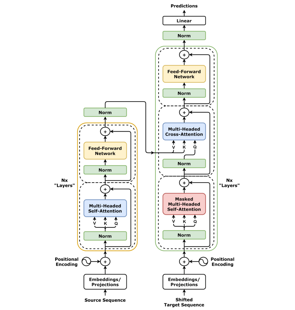
Transformer

GPT-OSS

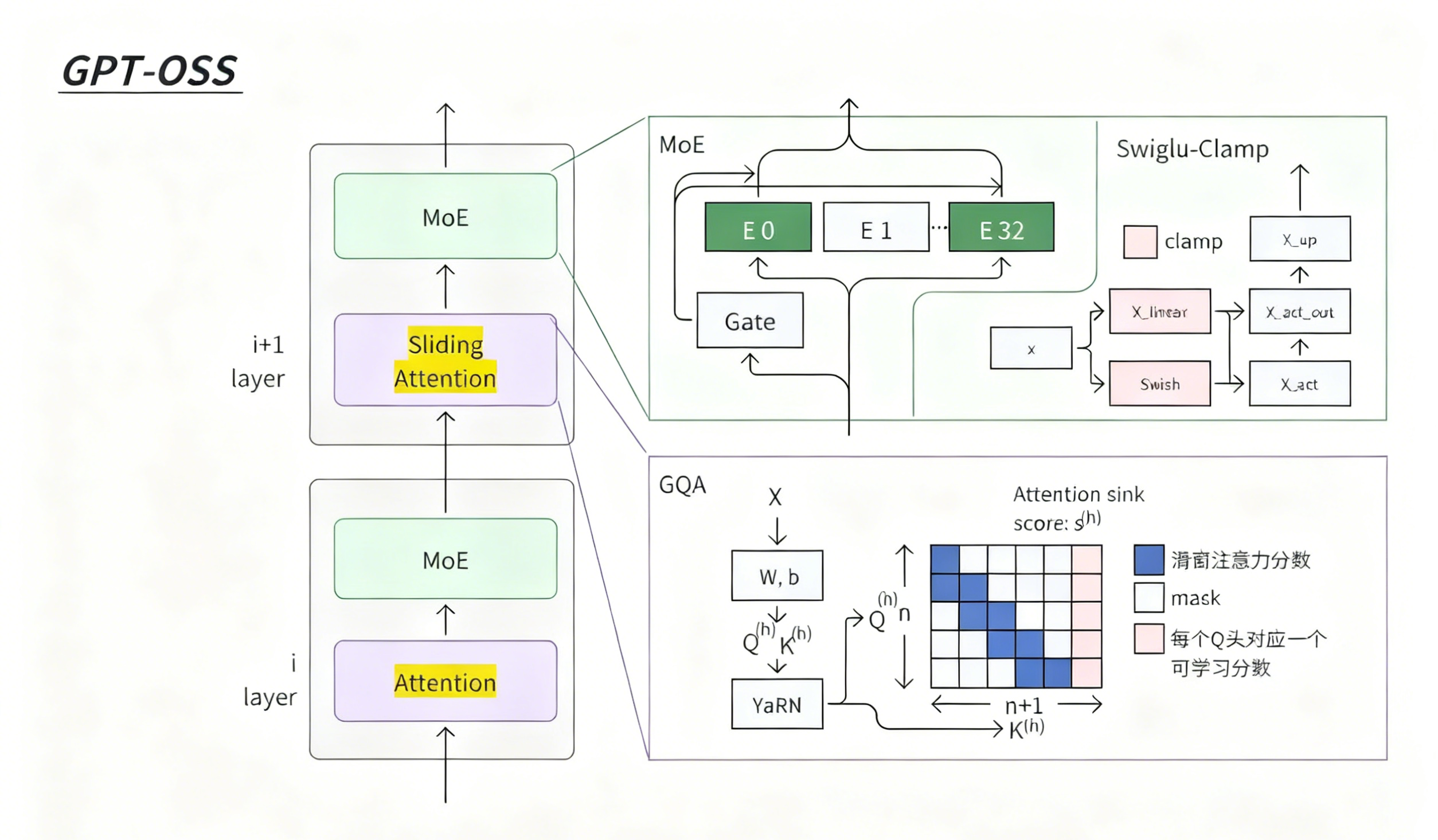
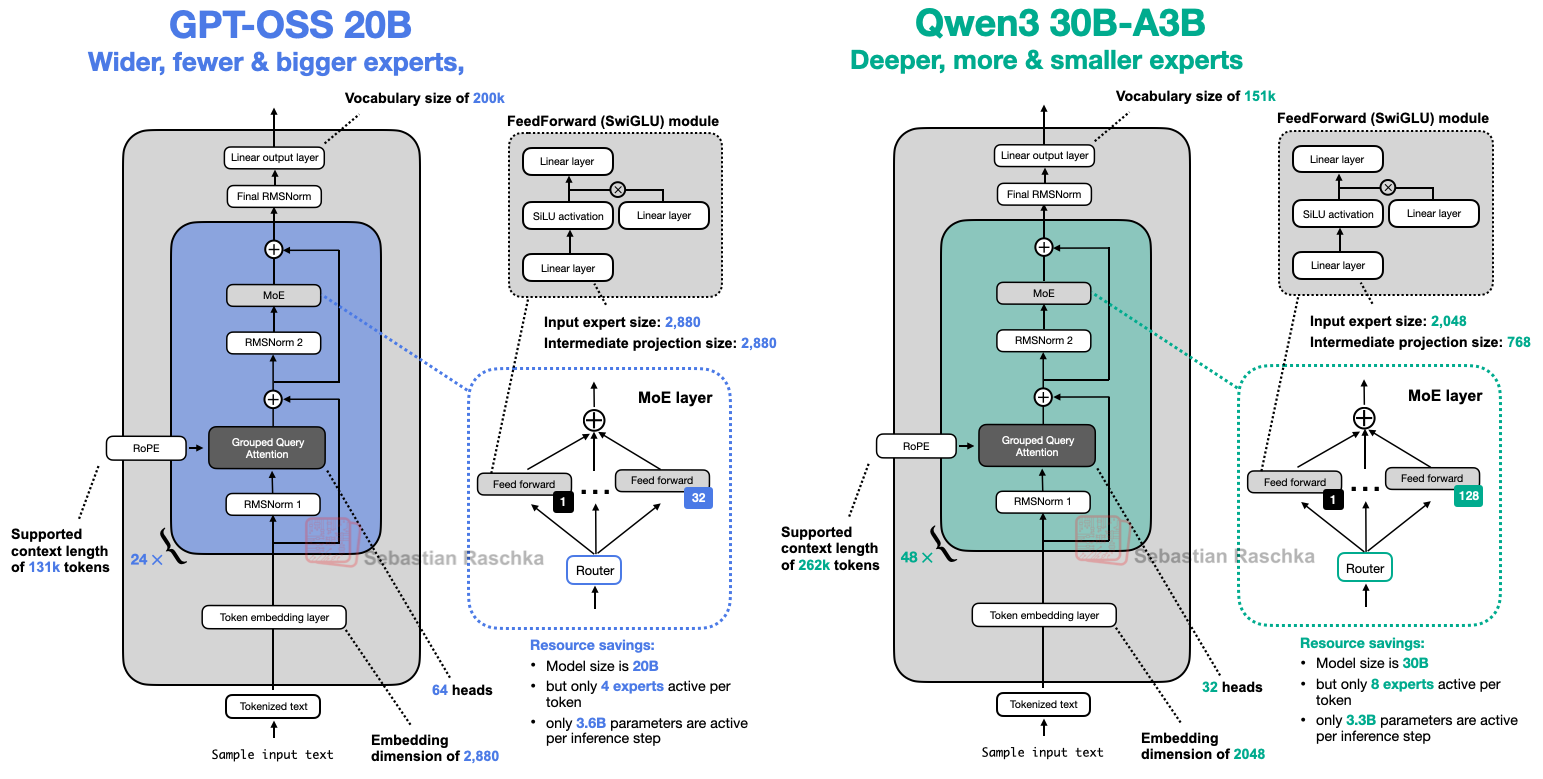
GPT-OSS是分层堆叠的设计，每一层（比如 i 层、i+1 层）都包含两个核心模块：
底层是Attention（注意力层），到了上层升级成Sliding Attention（滑动注意力）—— 这是为了处理超长文本时，减少计算量、提升效率。注意力层之上，都接了MoE（混合专家层）—— 也就是 “选专家” 模块，保证大模型能力的同时控制资源消耗。

模型对比

GPT-OSS源码解析

GPT-OSS源码目录结构

.
├── awesome-gpt-oss.md
├── _build
├── CMakeLists.txt
├── compatibility-test
├── docs
├── examples
├── gpt_oss
│   ├── chat.py
│   ├── evals
│   ├── generate.py
│   ├── __init__.py
│   ├── metal							# Metal后端（Apple CSilicon）
│   │   ├── benchmark
│   │   ├── CMakeLists.txt
│   │   ├── examples
│   │   ├── include
│   │   ├── __init__.py
│   │   ├── python
│   │   ├── scripts
│   │   ├── source
│   │   └── test
│   ├── responses_api				# API服务层
│   │   ├── api_server.py
│   │   ├── events.py
│   │   ├── inference				# 多后端推理接口
│   │   │   ├── __init__.py
│   │   │   ├── metal.py
│   │   │   ├── ollama.py
│   │   │   ├── stub.py
│   │   │   ├── transformers.py
│   │   │   ├── triton.py
│   │   │   └── vllm.py
│   │   ├── __init__.py
│   │   ├── serve.py
│   │   ├── types.py
│   │   └── utils.py
│   ├── tokenizer.py        # 统一分词器接口
│   ├── tools
│   ├── torch							# PyTorch后端（参考/分布式）
│   │   ├── __init__.py
│   │   ├── model.py				# 模型架构定义
│   │   ├── utils.py
│   │   └── weights.py			# 权重加载和量化处理
│   ├── triton						# Triton + CUDA后端（高性能）
│   │   ├── attention.py        # 注意力机制优化实现
│   │   ├── __init__.py
│   │   ├── model.py        # Triton 高性能推理实现，优化模型
│   │   └── moe.py      # Mixture of Experts (MoE) 实现
│   └── vllm			# vllm后端（张量并行）
│       └── token_generator.py
├── gpt-oss-mcp-server
├── LICENSE
├── MANIFEST.in
├── pyproject.toml
├── README.md
├── tests
├── tests-data
└── USAGE_POLICY

模型参数设置

@dataclass
class ModelConfig:
    num_hidden_layers: int = 36     # Transformer层数
    num_experts: int = 128          # MoE专家数量
    experts_per_token: int = 4      # 每个token激活的专家数
    vocab_size: int = 201088        # 词汇表大小
    hidden_size: int = 2880         # 隐藏层维度
    intermediate_size: int = 2880
    swiglu_limit: float = 7.0
    head_dim: int = 64              # 注意力头维度
    num_attention_heads: int = 64   # 注意力头数量
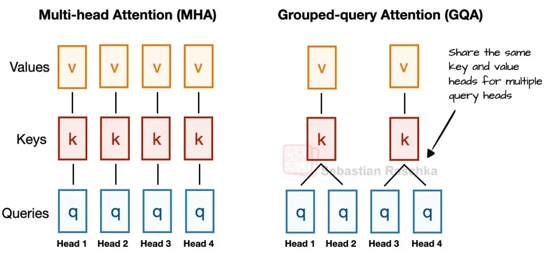
    num_key_value_heads: int = 8    # KV头数量(GQA)
    sliding_window: int = 128       # 滑动窗口大小
    initial_context_length: int = 4096
    rope_theta: float = 150000.0    # RoPE基础频率
    rope_scaling_factor: float = 32.0
    rope_ntk_alpha: float = 1.0
    rope_ntk_beta: float = 32.0

混合注意力机制

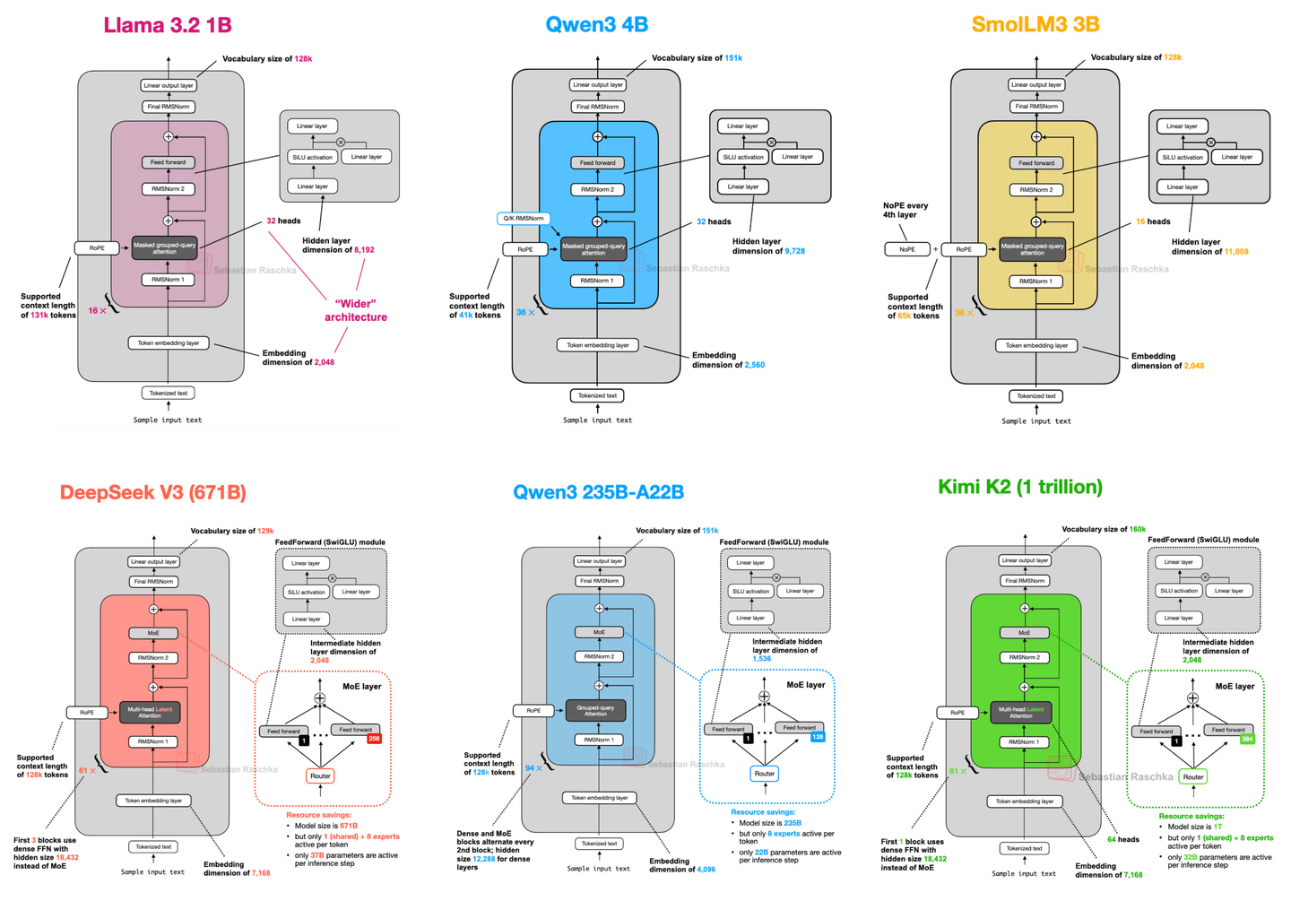
GPT-OSS采用了交替层设计策略，将滑动窗口注意力（Sliding Window Attention）和全注意力（Full Attention）有机结合。

在现代大语言模型（Large Language Model, LLM）的发展中，注意力机制（Attention Mechanism）一直是核心组件。然而，传统的全注意力机制（Full Attention）在处理长序列时面临着计算复杂度平方级增长的问题。GPT-OSS通过创新的混合注意力模式设计，在保持模型性能的同时显著降低了计算开销。

滑动窗口注意力机制

“滑动窗口注意力机制”—— 它是一种局部注意力机制，核心特点是 “每个位置只看自己周围固定范围的内容”。

在因果注意力也就是掩码注意力机制中，看到哪个词就会关注到前面所有的词。好处是能抓全信息，但如果文本很长，每个词都看所有前文，计算量会很大，就像 “看长篇小说时要回忆前几百章细节” 一样，又费时间又费精力。

而滑动窗口注意力就不一样，它只关注 “固定窗口内” 的前文 —— 比如这里窗口设得比较小，只关注前两个词，更早的词就给屏蔽掉了。
这其实特别像咱们看长篇小说的实际习惯：看到第 100 章时，不会硬记前 99 章的所有内容，只会重点回忆最近 5 章的情节 —— 既能快速跟上当前剧情（对应 “局部理解”），又不用耗费太多精力（对应 “节省计算力”）。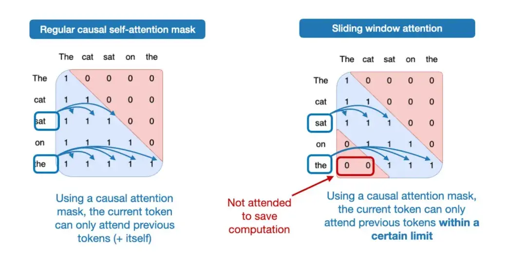

分组查询注意力

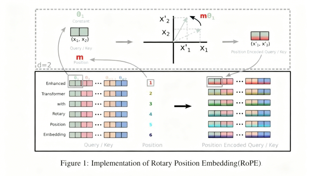
RoPE（旋转位置编码）则是通过绝对位置编码的方式实现相对位置编码。（结合了相对位置编码和绝对位置编码）

YARN（Yet Another RoPE extensioN）扩展是为了支持更长的序列。

RoPE位置编码与YARN扩展

pytorch后端

class AttentionBlock(torch.nn.Module):   # 注意力机制实现
    def __init__(
        self,
        config: ModelConfig,
        layer_idx: int = 0, 
        device: torch.device | None = None,
    ):
        super().__init__()
        self.head_dim = config.head_dim
        self.num_attention_heads = config.num_attention_heads
        self.num_key_value_heads = config.num_key_value_heads 
        # Only apply sliding window to every other layer
        self.sliding_window = config.sliding_window if layer_idx % 2 == 0 else 0
        self.sinks = torch.nn.Parameter(
            torch.empty(config.num_attention_heads, device=device, dtype=torch.bfloat16)
        )
        self.norm = RMSNorm(config.hidden_size, device=device)
        qkv_dim = config.head_dim * (
            config.num_attention_heads + 2 * config.num_key_value_heads
        )
        self.qkv = torch.nn.Linear(
            config.hidden_size, qkv_dim, device=device, dtype=torch.bfloat16
        )
        self.out = torch.nn.Linear(
            config.head_dim * config.num_attention_heads,
            config.hidden_size,
            device=device,
            dtype=torch.bfloat16,
        )
        self.sm_scale = 1 / math.sqrt(config.head_dim)
        self.rope = RotaryEmbedding(
            config.head_dim,
            config.rope_theta,
            torch.float32,
            initial_context_length=config.initial_context_length,
            scaling_factor=config.rope_scaling_factor,
            ntk_alpha=config.rope_ntk_alpha,
            ntk_beta=config.rope_ntk_beta,
            device=device,
        )

    def forward(self, x: torch.Tensor) -> torch.Tensor:   # 核心计算流程
        t = self.norm(x)   # RMSNorm归一化
        qkv = self.qkv(t)   # 一次性计算Q,K,V
        q = qkv[:, : self.num_attention_heads * self.head_dim].contiguous()
        k = qkv[
            :,
            self.num_attention_heads
            * self.head_dim : (self.num_attention_heads + self.num_key_value_heads)
            * self.head_dim,
        ].contiguous()
        v = qkv[
            :,
            (self.num_attention_heads + self.num_key_value_heads)
            * self.head_dim : (self.num_attention_heads + 2 * self.num_key_value_heads)
            * self.head_dim,
        ].contiguous()

        q = q.view(
            -1,
            self.num_key_value_heads,
            self.num_attention_heads // self.num_key_value_heads,
            self.head_dim,
        )
        k = k.view(-1, self.num_key_value_heads, self.head_dim)
        v = v.view(-1, self.num_key_value_heads, self.head_dim)
        q, k = self.rope(q, k)
        t = sdpa(q, k, v, self.sinks, self.sm_scale, self.sliding_window)   # 缩放点积注意力
        t = self.out(t)   # 输出投影
        t = x + t   # 残差连接
        return t

triton后端

class AttentionBlock(torch.nn.Module):
    def __init__(
        self,
        config: ModelConfig,
        layer_idx: int = 0,
        device: torch.device | None = None,
    ):
        super().__init__()
        self.head_dim = config.head_dim
        self.num_attention_heads = config.num_attention_heads
        self.num_key_value_heads = config.num_key_value_heads
        # Only apply sliding window to every other layer
        self.sliding_window = config.sliding_window if layer_idx % 2 == 0 else 0
        self.layer_idx = layer_idx
        self.sinks = torch.nn.Parameter(
            torch.empty(config.num_attention_heads, device=device, dtype=torch.bfloat16)
        )
        self.norm = RMSNorm(config.hidden_size, device=device)
        qkv_dim = config.head_dim * (
            config.num_attention_heads + 2 * config.num_key_value_heads
        )
        self.qkv = torch.nn.Linear(
            config.hidden_size, qkv_dim, device=device, dtype=torch.bfloat16
        )
        self.out = torch.nn.Linear(
            config.head_dim * config.num_attention_heads,
            config.hidden_size,
            device=device,
            dtype=torch.bfloat16,
        )
        self.sm_scale = 1 / math.sqrt(config.head_dim)
        self.rope = RotaryEmbedding(
            config.head_dim,
            config.rope_theta,
            torch.float32,
            initial_context_length=config.initial_context_length,
            scaling_factor=config.rope_scaling_factor,
            ntk_alpha=config.rope_ntk_alpha,
            ntk_beta=config.rope_ntk_beta,
            device=device,
        )

    @record_function("attn")
    def forward(self, x: torch.Tensor, cache: Cache | None = None) -> torch.Tensor:
        batch_size, n_ctx, dim = x.shape

        t = self.norm(x)
        with record_function("qkv"):
            qkv = self.qkv(t)
            qkv_parts = (
                self.num_attention_heads * self.head_dim,
                self.num_key_value_heads * self.head_dim,
                self.num_key_value_heads * self.head_dim
            )
            q, k, v = torch.split(qkv, qkv_parts, dim=-1)
            q, k, v = q.contiguous(), k.contiguous(), v.contiguous()

        q = q.view(batch_size, n_ctx, self.num_attention_heads, self.head_dim)
        k = k.view(batch_size, n_ctx, self.num_key_value_heads, self.head_dim)
        v = v.view(batch_size, n_ctx, self.num_key_value_heads, self.head_dim)

        if cache is not None:
            offset = cache.offset.clone()
            q, k = self.rope(q, k, offset=offset)
            k, v = cache.extend(k, v)
        else:
            offset = torch.zeros((1,), dtype=torch.long, device=x.device)
            q, k = self.rope(q, k, offset=offset)

        q = q.view(
            batch_size,
            n_ctx,
            self.num_attention_heads // self.num_key_value_heads,
            self.num_key_value_heads,
            self.head_dim,
        )
        with record_function("attn_kernel"):
            if n_ctx == 1:
                t = attention_ref(
                    q,
                    k,
                    v,
                    self.sinks,
                    self.sm_scale,
                    self.sliding_window,
                    offset,
                )
            else:
                t = attention(
                    q,
                    k,
                    v,
                    self.sinks,
                    self.sm_scale,
                    self.sliding_window,
                    offset,
                )
                if n_ctx < 64:
                    t1 = attention_ref(
                        q,
                        k,
                        v,
                        self.sinks,
                        self.sm_scale,
                        self.sliding_window,
                        offset,
                    )
                    torch.testing.assert_close(t, t1)
                    t = t1

        with record_function("c_proj"):
            t = self.out(t)
        t = x + t
        return t

MoE混合专家机制

MOE在现实大模型中的核心作用是在不显著增加计算成本的前提下，极大地扩展模型的总参数量，从而创造出能力更强、知识覆盖面更广的“专家型”模型。它通过一个智能路由系统，让每个输入只激活少量特定专家进行计算，实现了从“万亿参数模型”到“每次推理仅调用百亿参数”的高效转换，这使构建和部署超大规模模型在工程和商业上变得可行。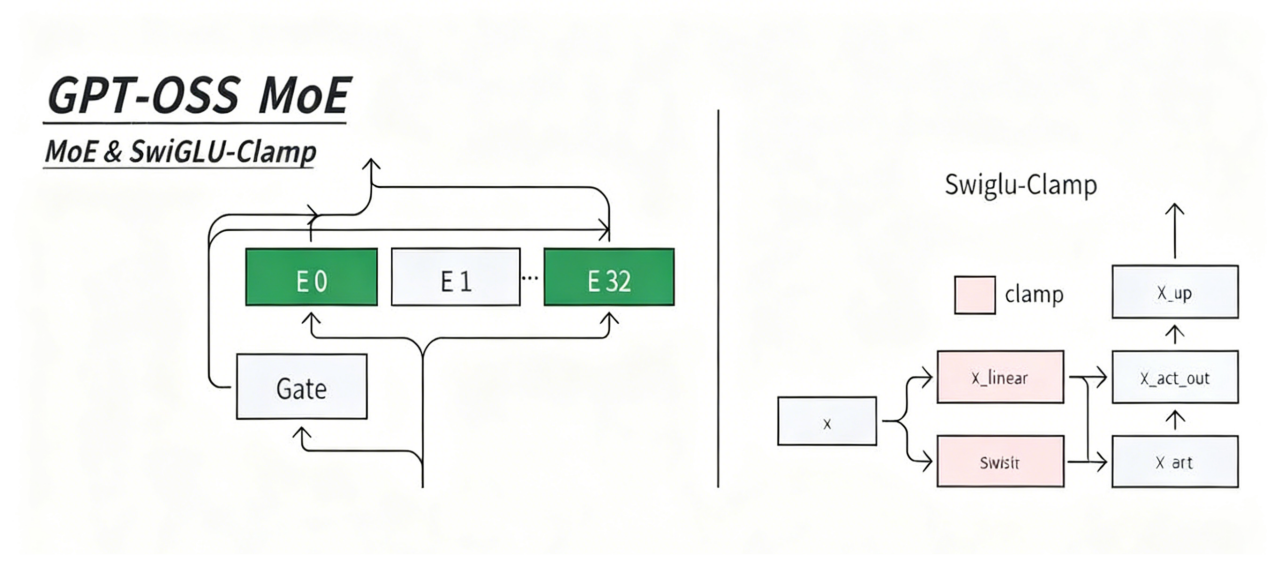

上图的 MoE&SwigLU-Clamp 部分是 MoE 层的内部逻辑。MoE 层靠Gate（门控）选专家（图里 E0 到 E32），只激活部分专家干活。每个专家内部用SwigLU-Clamp做前馈：在 SwigLU 的基础上加了 Clamp 操作，限制数值范围，让模型训练和推理更稳定。

pytorch后端

class MLPBlock(torch.nn.Module):
    def __init__(
        self,
        config: ModelConfig,
        device: torch.device | None = None,
    ):
        super().__init__()
        self.num_experts = config.num_experts
        self.experts_per_token = config.experts_per_token
        self.swiglu_limit = config.swiglu_limit
        self.world_size = dist.get_world_size() if dist.is_initialized() else 1
        self.norm = RMSNorm(config.hidden_size, device=device)
        self.gate = torch.nn.Linear(
            config.hidden_size, config.num_experts, device=device, dtype=torch.bfloat16
        )
        assert config.intermediate_size % self.world_size == 0
        self.mlp1_weight = torch.nn.Parameter(
            torch.empty(
                (
                    config.num_experts,
                    config.intermediate_size * 2 // self.world_size,
                    config.hidden_size,
                ),
                device=device,
                dtype=torch.bfloat16,
            )
        )
        self.mlp1_bias = torch.nn.Parameter(
            torch.empty(
                (config.num_experts, config.intermediate_size * 2 // self.world_size),
                device=device,
                dtype=torch.bfloat16,
            )
        )
        self.mlp2_weight = torch.nn.Parameter(
            torch.empty(
                (
                    config.num_experts,
                    config.hidden_size,
                    config.intermediate_size // self.world_size,
                ),
                device=device,
                dtype=torch.bfloat16,
            )
        )
        self.mlp2_bias = torch.nn.Parameter(
            torch.empty(
                (config.num_experts, config.hidden_size),
                device=device,
                dtype=torch.bfloat16,
            )
        )

    def forward(self, x: torch.Tensor) -> torch.Tensor:
        t = self.norm(x)
        g = self.gate(t)
        experts = torch.topk(g, k=self.experts_per_token, dim=-1, sorted=True)
        expert_weights = torch.nn.functional.softmax(experts.values, dim=1)
        expert_indices = experts.indices

        # MLP #1   # 扩展维度
        mlp1_weight = self.mlp1_weight[expert_indices, ...]
        mlp1_bias = self.mlp1_bias[expert_indices, ...]
        t = torch.einsum("beck,bk->bec", mlp1_weight, t) + mlp1_bias
        t = swiglu(t, limit=self.swiglu_limit)   # 激活函数

        # MLP #2   # 收缩维度
        mlp2_weight = self.mlp2_weight[expert_indices, ...]
        mlp2_bias = self.mlp2_bias[expert_indices, ...]
        t = torch.einsum("beck,bek->bec", mlp2_weight, t)
        if self.world_size > 1:
            dist.all_reduce(t, op=dist.ReduceOp.SUM)
        t += mlp2_bias   # 残差连接

        # Weighted sum of experts
        t = torch.einsum("bec,be->bc", t, expert_weights)

        return x + t

triton后端

def moe(x, wg, w1, w1_mx, w2, w2_mx, bg, b1, b2, experts_per_token=4, num_experts=128, swiglu_limit=7.0, fused_act=True, interleaved=True):
    if x.numel() == 0:
        return x

    pc1 = PrecisionConfig(weight_scale=w1_mx, flex_ctx=FlexCtx(rhs_data=InFlexData()))
    pc2 = PrecisionConfig(weight_scale=w2_mx, flex_ctx=FlexCtx(rhs_data=InFlexData()))
    pcg = PrecisionConfig(flex_ctx=FlexCtx(rhs_data=InFlexData()))

    # 1. Gate计算 - 决定使用哪些专家
    with record_function("wg"):
        logits = matmul_ogs(x, wg, bg, precision_config=pcg)

    # 2. 路由 - TopK专家选择
    with record_function("routing"):
        rdata, gather_indx, scatter_indx = routing(logits, experts_per_token, simulated_ep=1)

    # 3. 专家计算 - 第一层MLP + SwiGLU激活
    if fused_act:
        assert interleaved, "Fused activation requires interleaved weights"
        with record_function("w1+swiglu"):
            act = FusedActivation(FnSpecs("swiglu", triton_kernels.swiglu.swiglu_fn, ("alpha", "limit")), (1.702, swiglu_limit), 2)
            x = matmul_ogs(x, w1, b1, rdata, gather_indx=gather_indx, precision_config=pc1, fused_activation=act)
    else:
        with record_function("w1"):
            x = matmul_ogs(x, w1, b1, rdata, gather_indx=gather_indx, precision_config=pc1)
        with record_function("swiglu"):
            x = swiglu(x, limit=swiglu_limit, interleaved=interleaved)

    # 4. 专家计算 - 第二层MLP
    with record_function("w2"):
        x = matmul_ogs(x, w2, b2, rdata, scatter_indx=scatter_indx, precision_config=pc2, gammas=rdata.gate_scal)
    return x

激活函数

激活函数的核心作用是为模型注入非线性能力。

大模型的每一层的输入输出都是一个线性求和的过程，下一层的输出只是承接了上一层输入函数的线性变换，如果没有激活函数，线性层的计算只能得到线性结果，无论堆叠多少层，整个网络都等价于一个单层线性变换。

激活函数通过引入非线性变换，让神经网络能够强调重要的特征模式、抑制无关的噪声，组合出任意复杂的决策边界，从而让深度网络真正具备学习和推理的能力。它将基础的加权求和，升级为对复杂现实的拟合与理解，是模型获得智能的核心开关。

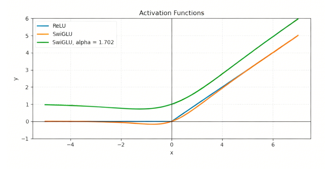
相对于其他大模型，GPT-OSS 激活函数的实现中使用了一个clamp函数。SwigLU 的输出可能会因为输入的波动出现 “特别大的正数” 或 “特别小的负数”，这些极端数值会让模型后续计算 “跑偏”（比如梯度爆炸、输出不稳定），clamp函数在这里是 “范围限制器”，作用是把 SwigLU 的输出控制在指定区间内，避免数值太夸张导致模型不稳定。

它的处理逻辑非常简单，需要设定一个最小值（min）和最大值（max）。当输入的数值小于 min 时，clamp 会把它强行改成 min；当输入的数值大于 max 时，clamp 会把它强行改成 max；数值在 min 和 max 之间时，保持不变。

pytorch后端

def swiglu(x, alpha: float = 1.702, limit: float = 7.0):
    x_glu, x_linear = x[..., ::2], x[..., 1::2]
    # Clamp the input values
    x_glu = x_glu.clamp(min=None, max=limit)
    x_linear = x_linear.clamp(min=-limit, max=limit)
    out_glu = x_glu * torch.sigmoid(alpha * x_glu)
    # Note we add an extra bias of 1 to the linear layer
    return out_glu * (x_linear + 1)

triton后端

def swiglu(x, alpha: float = 1.702, limit: float = 7.0, interleaved: bool = True):
    if interleaved:
        x_glu, x_linear = x[..., ::2], x[..., 1::2]   # 分离奇偶维度：将5760维分成两个2880维的路径
    else:
        x_glu, x_linear = torch.chunk(x, 2, dim=-1)
    x_glu = x_glu.clamp(min=None, max=limit)
    x_linear = x_linear.clamp(min=-limit, max=limit)
    out_glu = x_glu * torch.sigmoid(alpha * x_glu)   # 门控机制：一条路径学习"门"，另一条路径学习"内容"
    return out_glu * (x_linear + 1)   # 线性部分 + 门控部分   信息选择性通过：只有重要的信息才会被激活传递

均方根层归一化

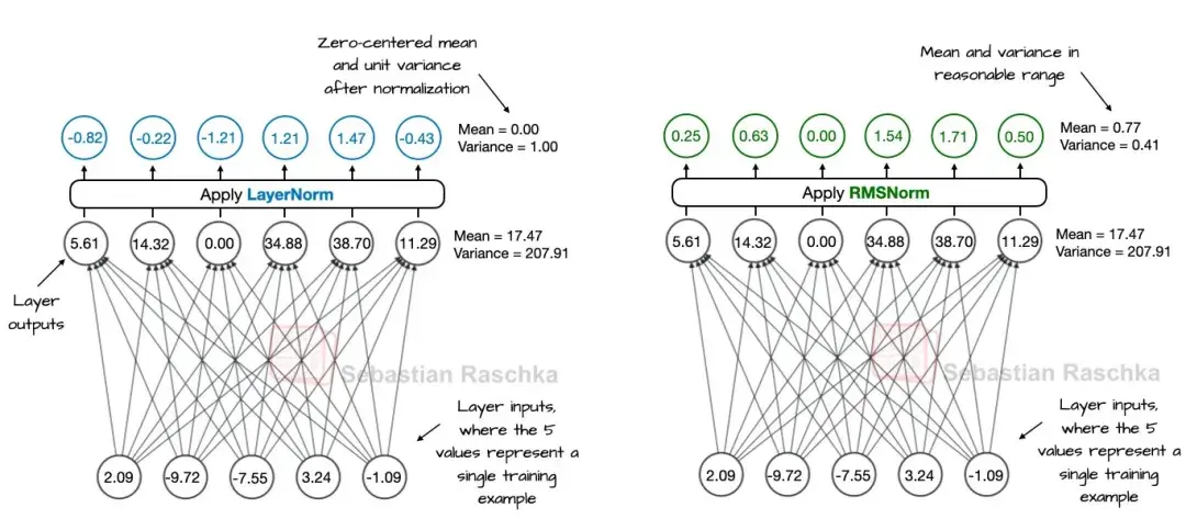
Normalization（归一化） 在机器学习和深度学习中是一种重要的数据预处理技术。它通过将输入数据或神经网络层的激活值限制在特定的范围内（如0到1之间），来加速训练收敛，防止梯度消失或爆炸，提高模型的泛化能力和数值稳定性。

常见的归一化方法包括Batch Normalization、Layer Normalization、Instance Normalization等。

GPT-OSS中使用的是均方根层归一化，它对同一组底层数据的处理更 “温和”—— 调整后均值是 0.77、方差 0.41，数值都落在合理范围里，但没有强行压成均值 0。相当于把 “参差不齐的队伍” 整理成 “松散但有序的队列”，保留了数据原有的一些趋势，同时又避免了极端值。（如下图右）

# pytorch和triton后端共用
class RMSNorm(torch.nn.Module):
    def __init__(
        self, num_features: int, eps: float = 1e-05, device: torch.device | None = None
    ):
        super().__init__()
        self.num_features = num_features
        self.eps = eps
        self.scale = torch.nn.Parameter(
            torch.ones(num_features, device=device, dtype=torch.float32)
        )

    def forward(self, x: torch.Tensor) -> torch.Tensor:
        assert x.shape[-1] == self.num_features
        t, dtype = x.float(), x.dtype
        t = t * torch.rsqrt(torch.mean(t**2, dim=-1, keepdim=True) + self.eps)
        return (t * self.scale).to(dtype)