CPT102小豪的笔记

自学笔记

小豪GO!

1569人浏览 · 2023-05-27 14:09:50

小豪GO! · 2023-05-27 14:09:50 发布

1. java的常用容器接口

1.1 Collection

Collection接口是Java集合框架的根接口，它定义了许多用于操作和管理集合的方法。Collection接口提供了一组通用的行为，可以用于操作各种类型的集合，如列表（List）、集（Set）和队列（Queue）等。

isEmpty(): 返回是否为空
size(): 返回已包含元素的数量
contains(E elem): 返回是否包含某个元素
add(E elem): 在尾部添加一个对象作为元素，返回操作状态
remove(E elem): 移除一个元素，返回操作状态
iterator()：返回一个迭代器
clear(): 利用迭代器清空集合
addall(Collection): 合并两Collection
removeAll(Collection): 移除所有位于两Collection交集里的所有元素
containsAll(Collection): 返回是否包含这个Collection的所有元素

1.2 List

继承自Collection

List的函数：

add()
clear()
size()
isEmpty()
get(i)
set(i,val)

1.3 Stack

stack没有接口只有实现，是一个类

push()
pop() (返回栈顶元素并删除)
peek()
empty()
clear()

1.4 Queue

Queue的接口要定义成Queue q = new LinkedList();

是Linkedlist的实现

add()
remove()删除并返回队头
isEmpty()
size()
clear()
peek()

priorityqueue是queue的实现，是一个优先队列，可以自定义优先级

默认是小根堆，在定义之后加coolections.reverseOrder()可以变成大根堆

1.5 Set

et接口的实现有Treeset(平衡树有序)和Hashset(无序)

Treeset 的增删查改都是logn的复杂度，而hashset是O(1)的复杂度实现treeset 定义变量要使用treeset：

TreeSet<Integer> ts = new TreeSet<Integer>();

Treeset里的两个函数:

ceiling和floor 分别返回大于等于key的最小元素和小于等于key的最大元素没有重复的元素

1.6 Map

HashMap
TreeMap

函数有：

put(key,value)
get(key)
containsKey(key)
remove(key) size()
isEmpty()
entrySet() 用来遍历map中的元素
Map.Entry<key, value> ：map中的对象类型

遍历map的代码

for(Map.Entry<Integer, Integer> entry : map.entrySet()) {
int key = entry.getKey();
int value = entry.getValue(); }

TreeMap中也有floorentry和ceilingentry函数

1.7 Abstraction

抽象数据结构，定义了一个数据结构的接口，数据结构的功能，不关心具体的实现可以映射到java的interface

比如 collection，list，set，queue，map

ArrayList，LinkedList，HashSet，TreeSet，PriorityQueue，HashMap，TreeMap 这些则是这些接口具体的实现

泛型 generic type 用来定义数据结构中储存的数据的类型，比如

ArrayList<Integer> al = new ArrayList<Integer>();

这样定义的arraylist只能储存integer类型的数据

Interfaces没有具体的构造器，所以不能直接new一个interface的对象，但是可以new一个interface的实现类的对象，比如

List<Integer> list = new ArrayList<Integer>();

ArrayList是一个具体的类，List是一个接口

1.8 Iterator

Iterator是Java集合框架中的一个接口，用于遍历集合中的元素。

所有Collection类都可以使用迭代器

List接口中的iterator()方法返回一个Iterator实例，用于遍历List中的元素。Iterator的实现包括以下方法：

hasNext(): 返回boolean值，表示集合中是否还有更多元素。

next(): 返回集合中的下一个元素。在调用此方法之前，应先调用hasNext()方法检查是否还有下一个元素。

remove(): 从集合中删除迭代器最近返回的元素。此方法在迭代过程中可以安全地修改集合。通常，在调用next()方法后调用此方法。

带有iterator的类型能够使用foreach循环，同时foreach循环就是iterator的另一种写法

for (Integer i : list) { System.out.println(i);
}
Iterator<Integer> it = list.iterator(); while (it.hasNext()) {
	System.out.println(it.next()); }
//自定义数据结构实现的iterator
	public class ARSet<T> implements Iterable<T> { private T[] items;
	private int size;

/**
* Create an empty set. */
@SuppressWarnings("unchecked") 
public ARSet() {
	items = (T[]) new Object[100]; size = 0;
}
private class ARSetIterator implements Iterator<T> { private int wizPos;

public ARSetIterator() {
	wizPos = 0; }

	@Override
	public boolean hasNext() {
		return wizPos < size }

		@Override
		public T next() {
			T returnItem = items[wizPos]; wizPos += 1;
			return returnItem; }
		}
	}
//类继承了Iterable接口之后，内部迭代器实现iterator方法

1.9 Comparable 和 Comparator

Comparable 和 Comparator 都是 Java 中用于比较对象的接口。这两者的主要区别在于它们的使用场景和实现方式。

所有Collection类都可以使用比较器

Comparable 是一个需要在要比较的对象类中实现的接口。如果类的实例具有自然顺序，如整数、字符串等，通常会实现 Comparable 接口。实现 Comparable 接口意味着类的对象可以与其他相同类型的对象进行比较。

Comparator 则是一个单独的接口，用于定义一种特定的比较规则。它通常用于在排序或搜索时自定义比较规则，而不必修改要比较的对象类。这在你无法修改原始类，或需要根据多种条件对对象进行排序时非常有用。

public class Person implements Comparable<Person> { 
	private String name;
	private int age;
	
	public Person(String name, int age) { this.name = name;
	this.age = age; }
	
	public String getName() { return name;
	}
	
	public int getAge() { return age;
	}
	
	@Override
	public String toString() {
		return "Person{name='" + name + "', age=" + age + "}"; }
	
		@Override
		public int compareTo(Person other) {
			return this.name.compareTo(other.name); }
		}

public class ComparableExample {
	public static void main(String[] args) {
		List<Person> people = new ArrayList<>();
		people.add(new Person("Alice", 30));
		people.add(new Person("Bob", 25));
		people.add(new Person("Charlie", 35));

		System.out.println("Before sorting by name: " + people);

		Collections.sort(people);

		System.out.println("After sorting by name: " + people);
	}
}
// 这是一个Comparable的例子

import java.util.Comparator;

public class AgeComparator implements Comparator<Person> {
	@Override
	public int compare(Person p1, Person p2) {
		return Integer.compare(p1.getAge(), p2.getAge());
	}
}

1.10 Tree

Java中的Tree（树）是一种常见的数据结构，它是由节点（Node）组成的层次结构。每个节点可以有零个或多个子节点，但每个节点只能有一个父节点（除了根节点）。树的一个重要特性是，从根节点到任何一个节点都存在唯一的路径。

在Java中，树的表示通常通过类和对象来实现。以下是一个简单的示例，展示如何在Java中表示一个树：

class TreeNode {
    private int data;
    private List<TreeNode> children;

    public TreeNode(int data) {
        this.data = data;
        this.children = new ArrayList<>();
    }

    public int getData() {
        return data;
    }

    public List<TreeNode> getChildren() {
        return children;
    }

    public void addChild(TreeNode child) {
        children.add(child);
    }
}

public class TreeExample {
    public static void main(String[] args) {
        // 创建树的节点
        TreeNode root = new TreeNode(1);
        TreeNode child1 = new TreeNode(2);
        TreeNode child2 = new TreeNode(3);
        TreeNode grandchild1 = new TreeNode(4);

        // 构建树的结构
        root.addChild(child1);
        root.addChild(child2);
        child1.addChild(grandchild1);

        // 遍历树
        traverseTree(root);
    }

    public static void traverseTree(TreeNode node) {
        System.out.println(node.getData());

        List<TreeNode> children = node.getChildren();
        for (TreeNode child : children) {
            traverseTree(child);
        }
    }
}

Java集合框架中的TreeSet和TreeMap，用于实现不同类型的树结构。

Terminology

Level: Equivalent to the “row” that a value is in
Depth: The number of levels in the tree
Leaf Nodes A node with no children
Non-leaf Nodes
Balanced: All leaf nodes are on levels n and (n+1), for some value of n (and are grouped on the bottom level “to the left”)

2. java的常用类

2.1 ArrayList

public class ArrayList<T> {
	private static final int DEFAULT_CAPACITY = 10;
	private T[] elements;
	private int size;

	public ArrayList() {
		elements = (T[]) new Object[DEFAULT_CAPACITY];
		size = 0;
	}

	public int size() {
		return size;
	}

	public boolean isEmpty() {
		return size == 0;
	}

	public T get(int index) {
		if (index < 0 || index >= size) {
			throw new IndexOutOfBoundsException("Invalid index: " + index);
		}
		return elements[index];
	}

	public void add(T item) {
		if (size == elements.length) {
			resize(2 * elements.length);
		}
		elements[size++] = item;
	}

	public T remove(int index) {
		if (index < 0 || index >= size) {
			throw new IndexOutOfBoundsException("Invalid index: " + index);
		}
		T item = elements[index];
		for (int i = index; i < size - 1; i++) {
			elements[i] = elements[i + 1];
		}
		size--;
		if (size > 0 && size == elements.length / 4) {
			resize(elements.length / 2);
		}
		return item;
	}

	private void resize(int newCapacity) {
		T[] newElements = (T[]) new Object[newCapacity];
		for (int i = 0; i < size; i++) {
			newElements[i] = elements[i];
		}
		elements = newElements;
	}
}

这个实现包括以下基本操作及其时间复杂度：

size()：返回列表中的元素数量。时间复杂度是 O(1)。isEmpty()：检查列表是否为空。时间复杂度是 O(1)。

get(int index)：获取列表中指定位置的元素。时间复杂度是 O(1)。

add(T item)：在列表末尾添加一个元素。平均时间复杂度是 O(1)，因为在数组需要扩容时会有 O(n) 的操作，但扩容操作的频率随着元素数量的增长而降低，根据均摊复杂度，该操作的复杂度仍为 O(1)。

remove(int index)：从列表中移除指定位置的元素。最坏情况下的时间复杂度是 O(n)，因为在移除元素后，可能需要将后续元素向前移动。类似地，在数组需要缩容时会有 O(n) 的操作，但这种情况发生的频率较低。

这个实现采用动态数组（数组大小可变）作为底层数据结构。当数组满时，它会自动扩大为原来的两倍；当数组元素数量小于四分之一时，它会缩小为原来的一半。这种自动调整大小的策略可以确保ArrayList 的空间效率。

注：这只是一个简化版的java底层ArrayList

提到了ensureCapacity这个方法，就是上面代码段的resize方法

Arraylist是一个动态长度的数组，在底层，它的这种动态长度其实由数组维护，一开始Arraylist是一个长度为4的数组，当被填满时，会触发他的扩容机制，本质上这个扩容机制是新建一个2*原本length长度的数组，然后将旧数组的元素复制到新数组中，然后将旧数组的引用指向新数组，这样就完成了扩容。这样的坏处是很可能会造成内存的浪费。

ArrayList和array的区别

动态性：ArrayList可以动态的增加和删除元素，而array的长度是固定的
类型：array只能储存一种基本数据类型的数据（如int，char等），而arraylist可以储存不同类型的数据（包括基本数据类型和引用对象类型，加上了泛型之后就只能储存一种特定的类型了）
性能：Array通常比ArrayList有更好的性能，因为Array没有使用额外的对象（如ArrayList的size、capacity等属性）和方法（如add、remove等），也不需要自动扩容。
内存使用：Array在内存上更紧凑，因为它不需要额外的内存来维护数据结构。ArrayList在内存上占用更多空间，因为它需要维护额外的属性和方法。

2.2 LinkedList

public class SinglyLinkedList<T> {
	private Node<T> head;
	private int size;

	private static class Node<T> {
		private T data;
		private Node<T> next;

		public Node(T data, Node<T> next) {
			this.data = data;
			this.next = next;
		}
	}

	public SinglyLinkedList() {
		head = null;
		size = 0;
	}

	public void addFirst(T item) {
		Node<T> newNode = new Node<>(item, head);

		head = newNode;
		size++;

	}

	public void addLast(T item) {
		Node<T> newNode = new Node<>(item,null);

		if (isEmpty()) {
			head = newNode;
		} else {
			Node<T> current = head;
			while (current.next != null) {
				current = current.next;
			}
			current.next = newNode;
		}
		size++;
	}

	public T removeFirst() {
		if (isEmpty()) {
			throw new RuntimeException("List is empty.");
		}
		T item = head.data;
		head = head.next;
		size--;
		return item;
	}

	public void insert(int index, T item) {
		if (index < 0 || index > size) {
			throw new IndexOutOfBoundsException("Invalid index: " + index);

		}

		if (index == 0) {
			addFirst(item);
			return;
		}

		Node<T> newNode = new Node<>(item,

				null);

		Node<T> current = head;

		for (int i = 0; i < index - 1; i++) {
			current = current.next;
		}

		newNode.next = current.next;
		current.next = newNode;
		size++;

	}

	public int size() {
		return size;
	}

	public boolean isEmpty()

	{
		return size == 0;
	}
}

此实现包含以下基本操作及其时间复杂度：

addFirst(item)：在链表头部添加一个元素。时间复杂度是 O(1)，因为只需将新节点添加到链表的头部，然后更新头部指针。

addLast(item)：在链表尾部添加一个元素。时间复杂度是 O(n)，因为需要遍历链表以找到尾部节点并添加新节点。

removeFirst()：从链表头部移除一个元素。时间复杂度是 O(1)，因为只需更新头部指针并返回移除的元素。

size()：返回链表中的元素数量。时间复杂度是 O(1)，因为我们使用了一个变量来维护链表大小。

isEmpty()：检查链表是否为空。时间复杂度是 O(1)，因为我们只需检查链表大小是否为0。

insert方法将一个元素插入到链表的指定位置。请注意，该方法在以下情况下的时间复杂度为：

插入元素到链表头部（index为0）：时间复杂度为 O(1)，因为只需将新节点添加到链表头部，然后更新头部指针。
插入元素到链表尾部（index为size）：时间复杂度为 O(n)，因为需要遍历链表以找到尾部节点并添加新节点。
插入元素到链表中间：时间复杂度为 O(n)，因为需要遍历链表以找到目标位置并插入新节点。

2.3 LinkedStack

public class LinkedStack<T> {
	private Node<T> top;
	private int size;

	private static class Node<T> {
		private T data;
		private Node<T> next;

		public Node(T data, Node<T> next) {
			this.data = data;
			this.next = next;
		}
	}

	public LinkedStack() {
		top = null;
		size = 0;
	}

	public void push(T item) {
		Node<T> newNode = new Node<>(item,

				top);

		top = newNode;
		size++;

	}

	public T pop() {
		if (isEmpty())

		{

			throw new RuntimeException("Stack is empty.");
		}
		T item = top.data;
		top = top.next;
		size--;
		return item;

	}

	public T peek() {
		if (isEmpty())

		{

			throw new RuntimeException("Stack is empty.");
		}
		return top.data;

	}

	public int size() {
		return size;
	}

	public boolean isEmpty()

	{

		return size == 0;
	}
}

以下是各个操作的时间复杂度分析：

push(item)：向堆栈顶部添加一个元素。时间复杂度是 O(1)，因为只需将新节点添加到链表的头部，然后更新头部指针。

pop()：从堆栈顶部移除一个元素。时间复杂度是 O(1)，因为只需更新头部指针并返回移除的元素。

peek()：查看堆栈顶部的元素，而不实际移除它。时间复杂度是 O(1)，因为只需返回头部节点的数据。

size()：返回堆栈中的元素数量。时间复杂度是 O(1)，因为我们使用了一个变量来维护堆栈大小。

isEmpty()：检查堆栈是否为空。时间复杂度是 O(1)，因为我们只需检查堆栈大小是否为0。

2.4 LinkedQueue

public class LinkedQueue<T> {
	private Node<T> front;
	private Node<T> rear;
	private int size;

	private static class Node<T> {
		private T data;
		private Node<T> next;

		public Node(T data, Node<T> next) {
			this.data = data;
			this.next = next;
		}
	}

	public LinkedQueue() {
		front = null;
		rear = null;
		size = 0;
	}

	public void enqueue(T item) {
		Node<T> newNode = new Node<>(item, null);
		if (isEmpty()) {
			front = newNode;
		} else {
			rear.next = newNode;
		}
		rear = newNode;
		size++;
	}

	public T dequeue() {
		if (isEmpty()) {
			throw new RuntimeException("Queue is empty.");
		}
		T item = front.data;
		front = front.next;
		if (front == null) {
			rear = null;
		}
		size--;
		return item;
	}

	public T peek() {
		if (isEmpty()) {
			throw new RuntimeException("Queue is empty.");
		}
		return front.data;
	}

	public int size() {
		return size;
	}

	public boolean isEmpty()

	{

		return size == 0;
	}
}

以下是各个操作的时间复杂度分析：

enqueue(item)：在队列尾部添加一个元素。时间复杂度是 O(1)，因为只需将新节点添加到链表的尾部，然后更新尾部指针。

dequeue()：从队列前端移除一个元素。时间复杂度是 O(1)，因为只需更新前端指针并返回移除的元素。

peek()：查看队列前端的元素，而不实际移除它。时间复杂度是 O(1)，因为只需返回前端节点的数据。

size()：返回队列中的元素数量。时间复杂度是 O(1)，因为我们使用了一个变量来维护队列大小。

isEmpty()：检查队列是否为空。时间复杂度是 O(1)，因为我们只需检查队列大小是否为0。

2.5 ArraySet

Arrayset是一个实现了Set接口的类，它的底层是一个array，所以它的元素是有序的，但是它的元素不能重复。

三个操作：

contains方法的时间复杂度是O(N)，因为它是遍历整个array来查找元素的。

Add(value)操作的时间复杂度是O(N)，因为它需要遍历整个array来查找是否已经存在value，如果不存在则添加到array的最后。

remove(value)操作的时间复杂度是O(N)，因为它需要遍历整个array来查找value，如果存在则删除。如何让ArraySet更快？

使用BinarySearch，但需要让Array是sorted的，所以需要在add的时候进行排序，这样add的时间复杂度就变成了O(NlogN)，但是contains的复杂度是O(logN)。

SortedArraySet

If you have to call add() and/or remove() many items, then SortedArraySet is no better than ArraySet

public SortedArraySet(Collection <E> col){ 
	// Make space
	count=col.size(); 
	data = (E[]) new Object[count]; 
	// Put items from collection into the data array. 
	col.toArray(data); 
	// sort the data array. 
	Arrays.sort(data); 
}

2.6 Tables (Maps)

indexed container
Associate information with a key – key is often a character string – info is any information
Typical Operations on Tables void insert(string key, Object o); object lookup(string key); void remove(string key);
Alternative implementations include
- Search Lists
- Binary Search Trees
- Hash Tables

2.7 Binary Search Tree

A binary search tree is a binary tree where each node has a key
The key in the left child (if exists) of a node is less than the key in the parent
The key in the right child (if exists) of a node is greater than the key in the parent
The left & right subtrees of the root are again binary search trees
for each node n, with key k
- n->left contains only nodes with keys < k
- n->right contains only nodes with keys > k
O(log N) in average for insert, lookup, and remove
operations can degenerate to O(N) – worst case!

2.8 AVL Trees (Adelson-Velskii and Landis)

A node is only allowed to possess one of three possible states:
Left-High (balance factor -1) The left-sub tree is one level taller than the right-sub tree
Balanced (balance factor 0) The left and right sub-trees both have the same heights
Right-High (balance factor +1) The right sub-tree is one level taller than the left-sub tree
If the balance of a node becomes -2 or +2 it will require rebalancing.
This is achieved by performing a rotation about this node
Rotation does not break the existing properties for a search tree

Algorithm	Average	Worst case
Search	O(log n)	O(log n)
Insert	O(log n)	O(log n)
Delete	O(log n)	O(log n)
Space	O(n)	O(n)

2.9 Binary Tree ADT

public interface BinaryTree<T> {
	BinaryTree<T> BinaryTree(T value);

	BinaryTree<T> getLeft();

	BinaryTree<T> getRight();

	void setLeft(BinaryTree<T> subtree);

	void setRight(BinaryTree<T> subtree);

	BinaryTree<T> find(T value);

	boolean contains(T value);

	boolean isEmpty();

	boolean isLeaf();

	int size();
}

2.10 Hash Tables

O(1) in average for insert, lookup, and remove
use an array named T of capacity N
define a hash function that returns an integer int H(string key)
must return an integer between 0 and N-1
store the key and info at T[H(key)]
H() must always return the same integer for a given key

Hash Function

A hash function is any well-defined procedure or mathematical function for turning data into an index into an array.
The values returned by a hash function are called hash values or simply hashes.
A hash function H is a transformation that
- takes a variable-size input k and
- returns a fixed-size string (or int), which is called the hash value h (that is, h = H(k))
In general, a hash function may map several different keys to the same hash value.

2.11 Binary Min-Heap

Binary Min-Heap（二叉最小堆）是一种基于完全二叉树的数据结构，其中每个节点的值都小于或等于其子节点的值。在二叉最小堆中，最小的元素位于根节点。

增加操作：

首先，将要插入的元素添加到堆的最后一个位置。
执行向上调整操作（也称为上浮操作）。从插入位置开始，将该元素与其父节点进行比较。如果当前元素小于其父节点，就将它与父节点交换位置。然后，将交换后的元素作为当前元素，继续向上比较和交换，直到满足二叉最小堆的性质为止。

删除操作：

首先，找到要删除的元素。为了保持二叉最小堆的性质，通常删除的是堆顶元素，即根节点。
将堆的最后一个元素移动到堆顶位置。将堆的最后一个元素替换为要删除的元素。
执行向下调整操作（也称为下沉操作）。从堆顶开始，与其两个子节点中较小的节点进行比较。如果当前节点大于子节点中的最小值，就将它与较小的子节点交换位置。然后，将交换后的节点作为当前节点，继续向下比较和交换，直到满足二叉最小堆的性质为止。

3. Graph

A graph G consist of :
- a finite set of vertices V(G), which cannot be empty,
- and a finite set of edges E(G), which connect pairs of vertices.
The number of vertices in G is called the order of G, denoted by |V|.
- Two vertices are adjacent if they are joined by an edge.
- Adjacent vertices are said to be neighbors.
- The edge which joins vertices is said to be incident to them
- Two or more edges joining the same pair of vertices are multiple edges.
- An edge joining a vertex to itself is called a loop.
- A graph containing no multiple edges or loops is called a simple graph

Degree

The number of times edges are incident to a vertex V is called its degree, denoted by d(V).
The degree sequence of a graph consists of the degrees of the vertices written in nonincreasing order, with repeats where necessary.
The sum of the values of the degrees, d(V), over all the vertices of a simple graph is twice the number of edges:

$\sum_{i} d\left(V_{i}\right)=2|E|$
A vertex of a digraph has an in-degree of d-(V) and an out-degree d+(V).

$\begin{array}{l} \sum_{i} d_{-}\left(V_{i}\right)=|A| \\ \sum_{i} d_{+}\left(V_{i}\right)=|A| \end{array}$

Subgraphs

A subgraph of G is a graph, H, whose vertex set is a subset of G’s vertex set, and whose edge set is a subset of the edge set of G.
If a subgraph H of G spans all of the vertices of G, i.e. V(H) = V(G), then H is called a spanning subgraph of G.

##3.1 Path

A sequence of edges of the form VsVi , ViVj , VjVk , VkVl , VlVt is a walk from Vs to Vt .
If these edges are distinct then the walk is called a trail, and
if the vertices are also distinct then the walk is called a path.
A walk or trail is closed if Vs = Vt .
A closed walk in which all the vertices are distinct except Vs and Vt , is called a cycle or a circuit.
The number of edges in a walk is called its length.

Connected graphs

A graph G is connected if there is a path from any one of its vertices to any other vertex.
A disconnected graph is said to be made up of components.

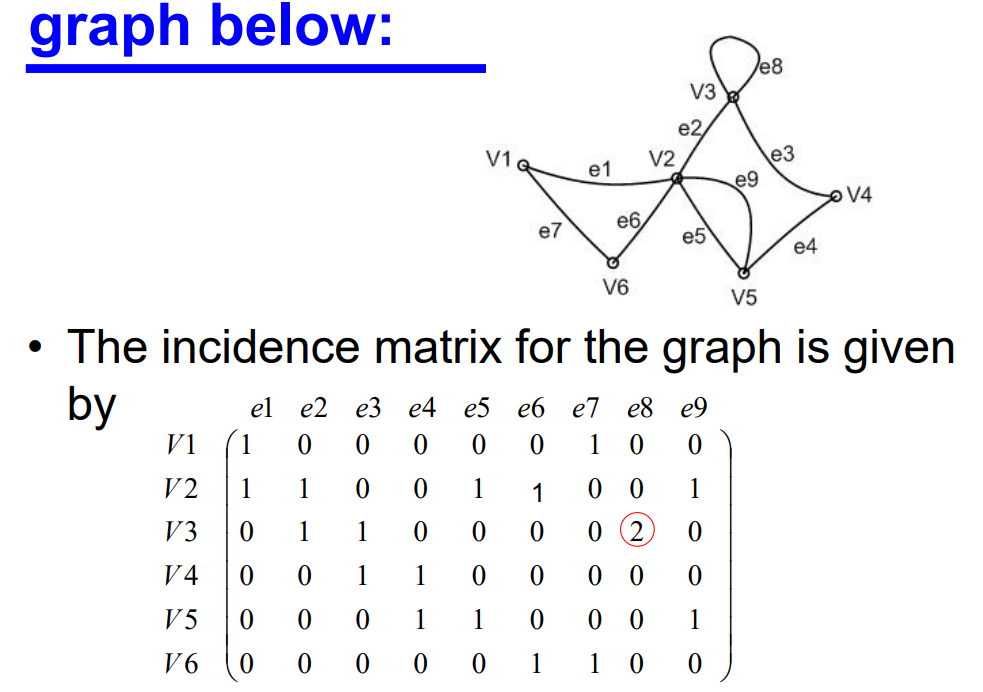
the incidence matrix

The incidence matrix of a graph G is a |V| × |E| matrix A.

The element aij = the number of times that vertex Vi is incident with the edge ej

在这里插入图片描述

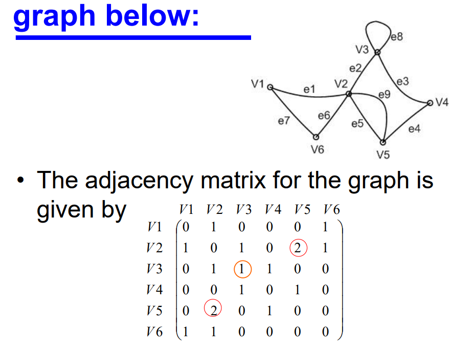
the adjacency matrix

The adjacency matrix of a graph G is a |V| × |V| matrix A.
The element aij = the number of edges joining Vi and Vj

4. Trees and forests

A tree is a connected graph with no cycles.
A forest is a graph with no cycles and it may or may not be connected
If a tree T has at least two vertices then it has the following properties:
There is exactly one path from any vertex Vi in T to any other vertex Vj
The graph obtained from tree T by removing any edge has two components, each of which is a tree.
|E| = |V| - 1

2048 AI社区

有“AI”的1024 = 2048，欢迎大家加入2048 AI社区

更多推荐

Conda与Poetry：构建可复现、无冲突的Python环境

2048 AI社区

解读ISO IEC 23053-2022

该摘要概述了ISO/IEC23053-2022标准的核心内容与价值。标准旨在为基于机器学习的AI系统建立统一术语和通用框架，明确区分ML模型与ML系统的概念，并定义系统开发生命周期的关键阶段（需求分析、数据工程、模型训练、系统集成、部署运维等）。其核心价值在于促进AI领域的互操作性、提高透明度、指导风险管理，并为后续细分标准奠定基础。该框架适用于AI项目管理、系统设计、教育培训及政策制定等场景，是