个人CNN学习记录之VGG网络

---

---

前言

在日常工作中，我专注于并行计算领域，主要依托GPGPU、NPU等高算力芯片进行开发。当前，高算力与AI已深度融合，计算与人工智能二者相辅相成：底层计算为实现通用算法与算子提供基础，而AI模型则能反哺并优化传统算法的决策效率与性能。为系统构建这方面的知识体系，我在公司导师的推荐下，跟随up主“霹雳吧啦Wz”的CNN系列视频进行学习，并通过博客记录学习过程，融入自己的理解与总结。

一、VGG网络介绍

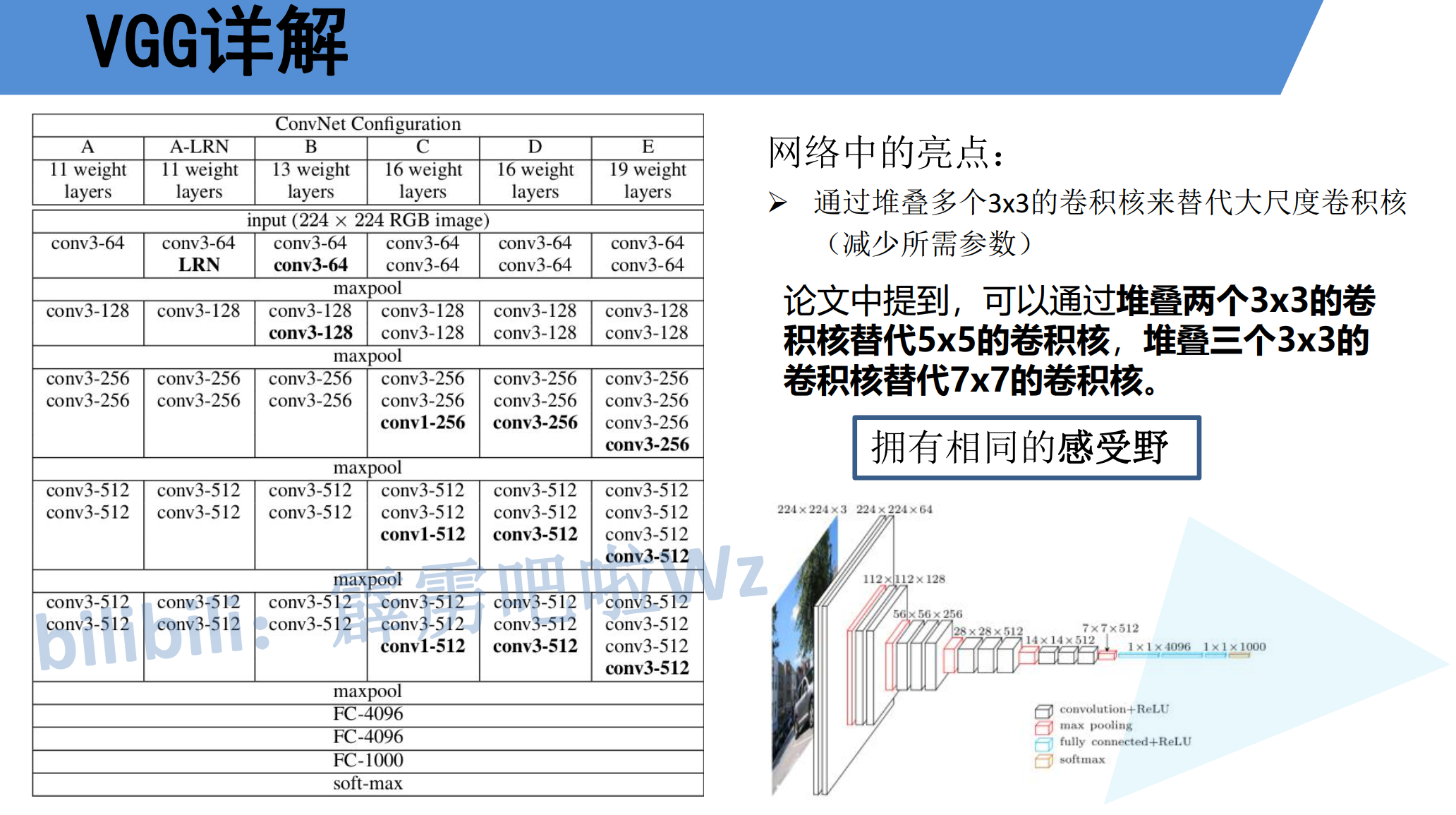
图中展示了VGG网络的基本架构，展示了很多种配置，分别在深度、是否使用LRN都做了各种尝试。最常用的配置是D配置，这个16层结构。

网络中的亮点：
使用多个连续的、尺寸更小的3×3卷积核，来替代传统网络中较大的卷积核（如5×5、7×7）。

优势：
大幅减少参数量：这是最直接的优点。例如，一个5×5卷积层的参数量是 5 * 5C_inC_out = 25C_inC_out。而用两个3×3卷积层达到相同感受野时，参数量为 2*(3 * 3C_inC_out) = 18C_inC_out，参数减少了28%。层数越深、通道数越多，节省的量越显著。

增加网络深度与非线性的：堆叠的小卷积核在保持相同感受野的同时，增加了网络的深度。更深的网络可以学习更复杂的特征。同时，每个卷积层后都跟随一个ReLU激活函数，这引入了更多的非线性变换，增强了模型的表达能力。

拥有相同的感受野：图片右侧明确指出了这一点。两个3×3卷积堆叠的感受野是5×5，三个3×3卷积堆叠的感受野是7×7。这使得VGG能够在更深、更复杂的同时，捕捉到与使用大卷积核时同样范围的图像信息。

二、感受野

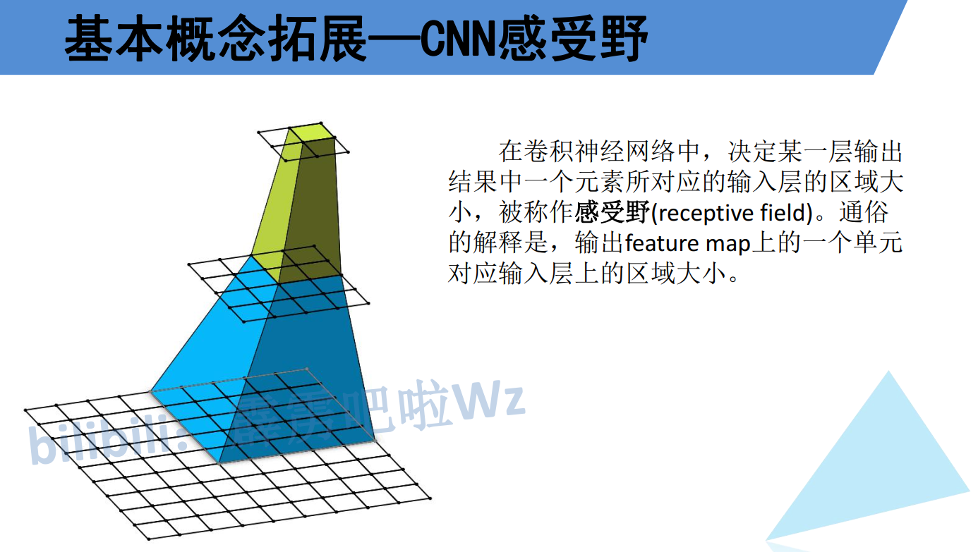
感受野标准定义：在卷积神经网络中，决定某一层输出结果中一个元素所对应的输入层的区域大小，被称作感受野。

通俗解释：输出特征图（feature map）上的一个“单元”（或像素点），是由输入层上多大范围的区域计算得出的。这个区域就是该单元的感受野。

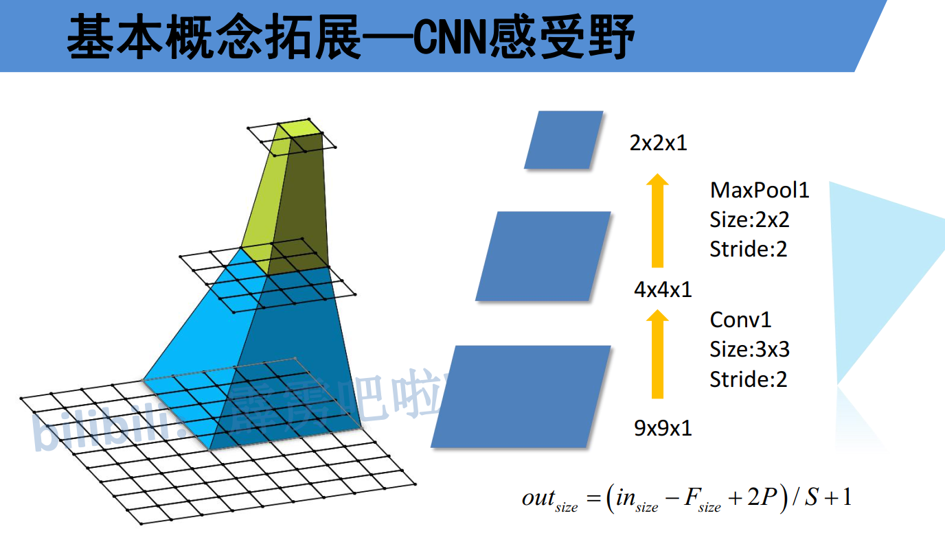
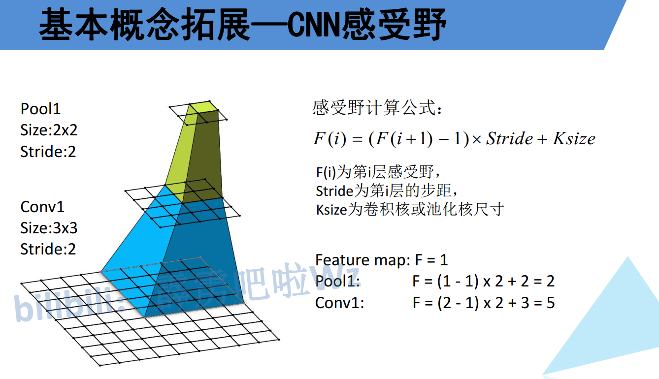
图片给出了计算感受野的标准递推公式：
F(i) = ( F(i+1) - 1 ) × Stride + Ksize
F(i)：第 i层的感受野（我们想求的值）。
F(i+1)：第 i+1层的感受野（后一层的值，是计算的起点）。
Stride：第 i层的步长（Stride）。
Ksize：第 i层的卷积核或池化核尺寸（Kernel Size）。

公式理解：要计算当前层 i的感受野，需要知道它后面一层 i+1的感受野有多大，然后根据本层的“步伐”（Stride）和“视野宽度”（Ksize）进行放大。这是一个从网络输出层向输入层反向递推的过程。

计算示例解析（对应图中右半部分）

图片通过一个具体例子演示了如何应用公式：
起点：从网络的末端（最终的特征图）开始。假设最后一层 Feature Map的一个点，只对应自己，所以其感受野 F = 1。

计算 Pool1层的感受野：

已知：Pool1的下一层（即Feature Map）的感受野 F(i+1) = 1。

Pool1层的参数：Ksize = 2（池化核2x2），Stride = 2（步长为2）。

代入公式：F(Pool1) = (1 - 1) × 2 + 2 = 2。

结论：Pool1层特征图上的一个点，对应其输入（即Conv1层输出）上 2×2​ 的区域。

计算 Conv1层的感受野：

已知：Conv1的下一层（即Pool1）的感受野 F(i+1) = 2。

Conv1层的参数：Ksize = 3（卷积核3x3），Stride = 2（步长为2）。

代入公式：F(Conv1) = (2 - 1) × 2 + 3 = 5。

最终结论：Conv1层特征图上的一个点，对应原始输入图像上 5×5​ 的区域。这就是本例中 Conv1层的感受野。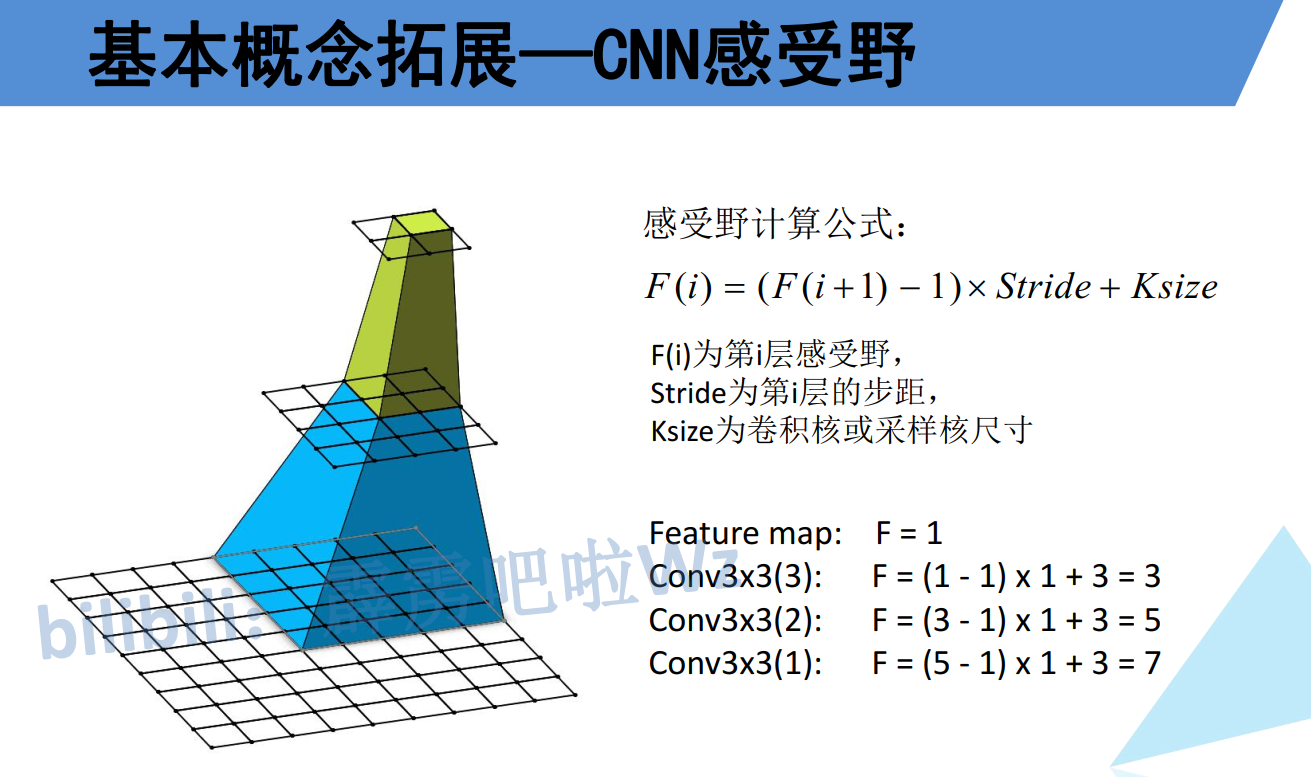

按照同样的逻辑计算3个3x3卷积层堆叠后的感受野，结果发现3个33的卷积核和一个77的卷积核的感受野相同。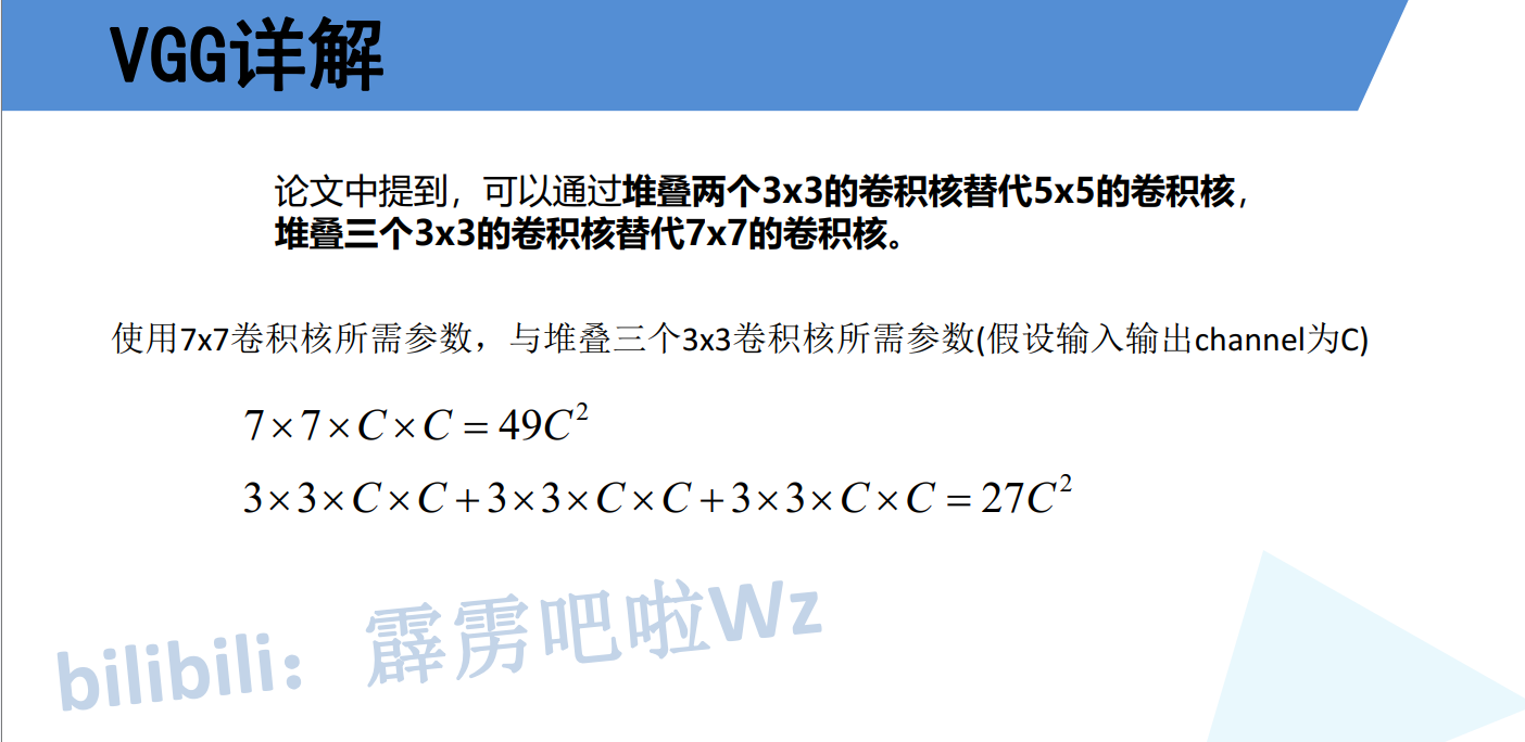

虽然感受野相同，但计算参数却减少了一半

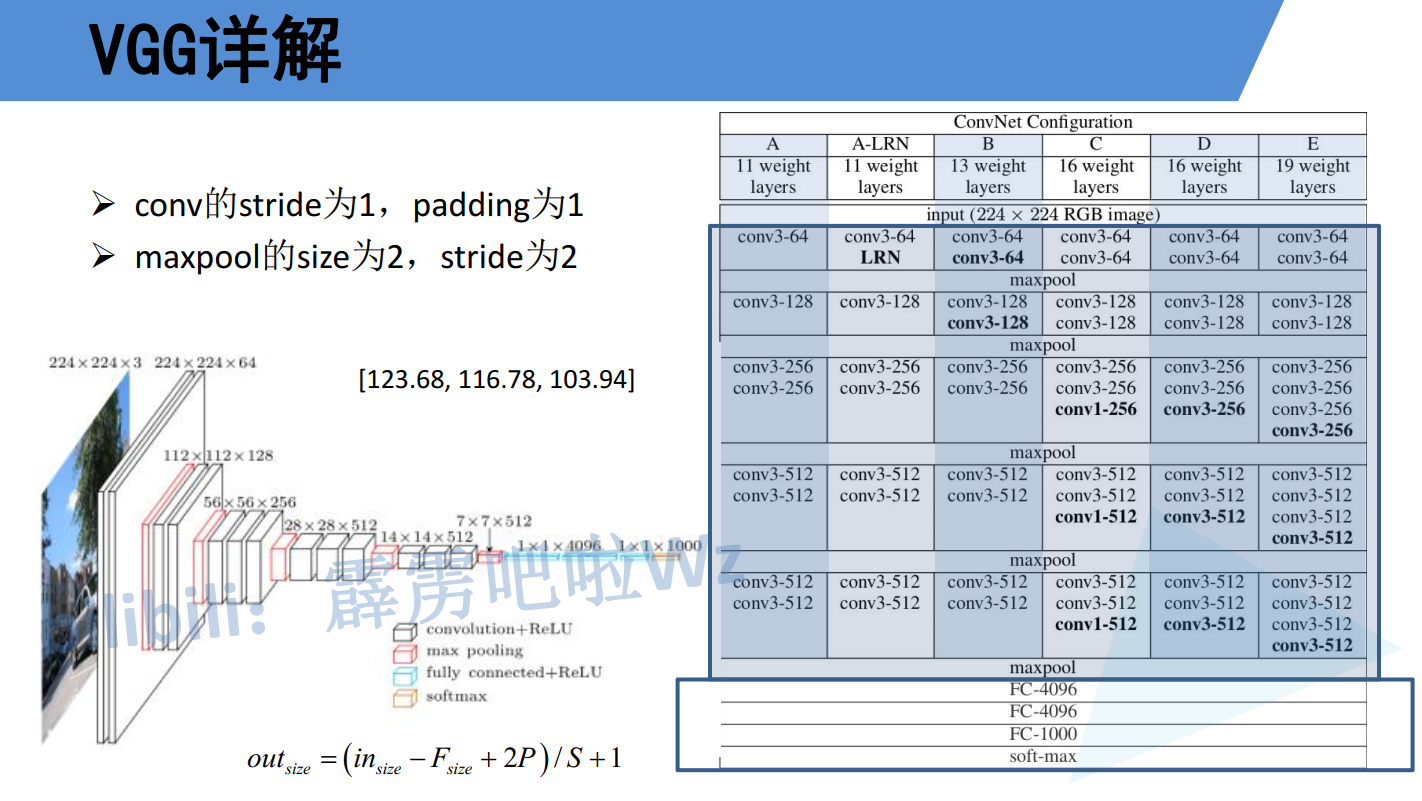
最后对VGG网络架构做了阐述，按照D的配置，图中各层架构写的比较详细。这里文本不做阐述。

三、代码分析

model.py

import torch.nn as nn
import torch

# official pretrain weights
model_urls = {
    'vgg11': 'https://download.pytorch.org/models/vgg11-bbd30ac9.pth',
    'vgg13': 'https://download.pytorch.org/models/vgg13-c768596a.pth',
    'vgg16': 'https://download.pytorch.org/models/vgg16-397923af.pth',
    'vgg19': 'https://download.pytorch.org/models/vgg19-dcbb9e9d.pth'
}


class VGG(nn.Module):
    def __init__(self, features, num_classes=1000, init_weights=False):
        super(VGG, self).__init__()
        self.features = features
        self.classifier = nn.Sequential(
            nn.Linear(512*7*7, 4096),
            nn.ReLU(True),
            nn.Dropout(p=0.5),
            nn.Linear(4096, 4096),
            nn.ReLU(True),
            nn.Dropout(p=0.5),
            nn.Linear(4096, num_classes)
        )
        if init_weights:
            self._initialize_weights()

    def forward(self, x):
        # N x 3 x 224 x 224
        x = self.features(x)
        # N x 512 x 7 x 7
        x = torch.flatten(x, start_dim=1)
        # N x 512*7*7
        x = self.classifier(x)
        return x

    def _initialize_weights(self):
        for m in self.modules():
            if isinstance(m, nn.Conv2d):
                # nn.init.kaiming_normal_(m.weight, mode='fan_out', nonlinearity='relu')
                nn.init.xavier_uniform_(m.weight)
                if m.bias is not None:
                    nn.init.constant_(m.bias, 0)
            elif isinstance(m, nn.Linear):
                nn.init.xavier_uniform_(m.weight)
                # nn.init.normal_(m.weight, 0, 0.01)
                nn.init.constant_(m.bias, 0)


def make_features(cfg: list):
    layers = []
    in_channels = 3
    for v in cfg:
        if v == "M":
            layers += [nn.MaxPool2d(kernel_size=2, stride=2)]
        else:
            conv2d = nn.Conv2d(in_channels, v, kernel_size=3, padding=1)
            layers += [conv2d, nn.ReLU(True)]
            in_channels = v
    return nn.Sequential(*layers)


cfgs = {
    'vgg11': [64, 'M', 128, 'M', 256, 256, 'M', 512, 512, 'M', 512, 512, 'M'],
    'vgg13': [64, 64, 'M', 128, 128, 'M', 256, 256, 'M', 512, 512, 'M', 512, 512, 'M'],
    'vgg16': [64, 64, 'M', 128, 128, 'M', 256, 256, 256, 'M', 512, 512, 512, 'M', 512, 512, 512, 'M'],
    'vgg19': [64, 64, 'M', 128, 128, 'M', 256, 256, 256, 256, 'M', 512, 512, 512, 512, 'M', 512, 512, 512, 512, 'M'],
}


def vgg(model_name="vgg16", **kwargs):
    assert model_name in cfgs, "Warning: model number {} not in cfgs dict!".format(model_name)
    cfg = cfgs[model_name]

    model = VGG(make_features(cfg), **kwargs)
    return model

相较以前博客分析的Lenet、AlexNlet代码来看没什么太大的变化，这里用了点代码层面的小技巧，通过cfgs把各种VGG网络配置参数通过结构体数组显性化，在make_features制作特征提取网络时根据参数来搭建对应的卷积层和池化层。

train.py

import os
import sys
import json

import torch
import torch.nn as nn
from torchvision import transforms, datasets
import torch.optim as optim
from tqdm import tqdm

from model import vgg


def main():
    device = torch.device("cuda:0" if torch.cuda.is_available() else "cpu")
    print("using {} device.".format(device))

    data_transform = {
        "train": transforms.Compose([transforms.RandomResizedCrop(224),
                                     transforms.RandomHorizontalFlip(),
                                     transforms.ToTensor(),
                                     transforms.Normalize((0.5, 0.5, 0.5), (0.5, 0.5, 0.5))]),
        "val": transforms.Compose([transforms.Resize((224, 224)),
                                   transforms.ToTensor(),
                                   transforms.Normalize((0.5, 0.5, 0.5), (0.5, 0.5, 0.5))])}

    data_root = os.path.abspath(os.path.join(os.getcwd(), "../.."))  # get data root path
    image_path = os.path.join(data_root, "data_set", "flower_data")  # flower data set path
    assert os.path.exists(image_path), "{} path does not exist.".format(image_path)
    train_dataset = datasets.ImageFolder(root=os.path.join(image_path, "train"),
                                         transform=data_transform["train"])
    train_num = len(train_dataset)

    # {'daisy':0, 'dandelion':1, 'roses':2, 'sunflower':3, 'tulips':4}
    flower_list = train_dataset.class_to_idx
    cla_dict = dict((val, key) for key, val in flower_list.items())
    # write dict into json file
    json_str = json.dumps(cla_dict, indent=4)
    with open('class_indices.json', 'w') as json_file:
        json_file.write(json_str)

    batch_size = 32
    nw = min([os.cpu_count(), batch_size if batch_size > 1 else 0, 8])  # number of workers
    print('Using {} dataloader workers every process'.format(nw))

    train_loader = torch.utils.data.DataLoader(train_dataset,
                                               batch_size=batch_size, shuffle=True,
                                               num_workers=nw)

    validate_dataset = datasets.ImageFolder(root=os.path.join(image_path, "val"),
                                            transform=data_transform["val"])
    val_num = len(validate_dataset)
    validate_loader = torch.utils.data.DataLoader(validate_dataset,
                                                  batch_size=batch_size, shuffle=False,
                                                  num_workers=nw)
    print("using {} images for training, {} images for validation.".format(train_num,
                                                                           val_num))

    # test_data_iter = iter(validate_loader)
    # test_image, test_label = test_data_iter.next()

    model_name = "vgg16"
    net = vgg(model_name=model_name, num_classes=5, init_weights=True)
    net.to(device)
    loss_function = nn.CrossEntropyLoss()
    optimizer = optim.Adam(net.parameters(), lr=0.0001)

    epochs = 30
    best_acc = 0.0
    save_path = './{}Net.pth'.format(model_name)
    train_steps = len(train_loader)
    for epoch in range(epochs):
        # train
        net.train()
        running_loss = 0.0
        train_bar = tqdm(train_loader, file=sys.stdout)
        for step, data in enumerate(train_bar):
            images, labels = data
            optimizer.zero_grad()
            outputs = net(images.to(device))
            loss = loss_function(outputs, labels.to(device))
            loss.backward()
            optimizer.step()

            # print statistics
            running_loss += loss.item()

            train_bar.desc = "train epoch[{}/{}] loss:{:.3f}".format(epoch + 1,
                                                                     epochs,
                                                                     loss)

        # validate
        net.eval()
        acc = 0.0  # accumulate accurate number / epoch
        with torch.no_grad():
            val_bar = tqdm(validate_loader, file=sys.stdout)
            for val_data in val_bar:
                val_images, val_labels = val_data
                outputs = net(val_images.to(device))
                predict_y = torch.max(outputs, dim=1)[1]
                acc += torch.eq(predict_y, val_labels.to(device)).sum().item()

        val_accurate = acc / val_num
        print('[epoch %d] train_loss: %.3f  val_accuracy: %.3f' %
              (epoch + 1, running_loss / train_steps, val_accurate))

        if val_accurate > best_acc:
            best_acc = val_accurate
            torch.save(net.state_dict(), save_path)

    print('Finished Training')


if __name__ == '__main__':
    main()

训练脚本相较以前博客分析的Lenet、AlexNlet代码来看没什么太大的变化，这里不做分析

predict.py

import os
import json

import torch
from PIL import Image
from torchvision import transforms
import matplotlib.pyplot as plt

from model import vgg


def main():
    device = torch.device("cuda:0" if torch.cuda.is_available() else "cpu")

    data_transform = transforms.Compose(
        [transforms.Resize((224, 224)),
         transforms.ToTensor(),
         transforms.Normalize((0.5, 0.5, 0.5), (0.5, 0.5, 0.5))])

    # load image
    img_path = "../tulip.jpg"
    assert os.path.exists(img_path), "file: '{}' dose not exist.".format(img_path)
    img = Image.open(img_path)
    plt.imshow(img)
    # [N, C, H, W]
    img = data_transform(img)
    # expand batch dimension
    img = torch.unsqueeze(img, dim=0)

    # read class_indict
    json_path = './class_indices.json'
    assert os.path.exists(json_path), "file: '{}' dose not exist.".format(json_path)

    with open(json_path, "r") as f:
        class_indict = json.load(f)
    
    # create model
    model = vgg(model_name="vgg16", num_classes=5).to(device)
    # load model weights
    weights_path = "./vgg16Net.pth"
    assert os.path.exists(weights_path), "file: '{}' dose not exist.".format(weights_path)
    model.load_state_dict(torch.load(weights_path, map_location=device))

    model.eval()
    with torch.no_grad():
        # predict class
        output = torch.squeeze(model(img.to(device))).cpu()
        predict = torch.softmax(output, dim=0)
        predict_cla = torch.argmax(predict).numpy()

    print_res = "class: {}   prob: {:.3}".format(class_indict[str(predict_cla)],
                                                 predict[predict_cla].numpy())
    plt.title(print_res)
    for i in range(len(predict)):
        print("class: {:10}   prob: {:.3}".format(class_indict[str(i)],
                                                  predict[i].numpy()))
    plt.show()


if __name__ == '__main__':
    main()

预测脚本相较以前博客分析的Lenet、AlexNlet代码来看没什么太大的变化，这里也不做分析。

---

总结

以上就是今天要讲的内容