一文搞懂CLIP模型!CLIP 论文逐段精读及网络结构源码解析
CLIP 论文逐段精读 + 网络结构源码解析
原论文:Learning Transferable Visual Models From Natural Language Supervision(https://arxiv.org/pdf/2103.00020.pdf)
arXiv: 2103.00020 | OpenAI 2021
本文档:每段附原文英文 → 中文逐句解读 → 深层含义分析;最后完整拆解模型结构与维度变化
目录
- Abstract(摘要)
- Section 1: Introduction and Motivating Work(引言)
- Section 2.1: Natural Language Supervision(自然语言监督)
- Section 2.2: Creating a Sufficiently Large Dataset(数据集构建)
- Section 2.3: Selecting an Efficient Pre-Training Method(预训练方法选择)
- Section 2.4: Choosing and Scaling a Model(模型选择与扩展)
- Section 2.5: Training(训练细节)
- Section 3.1: Zero-Shot Transfer(零样本迁移)
- Section 3.2: Prompt Engineering(提示工程)
- Section 3.4: Robustness(鲁棒性)
- Section 4: Human Comparison(与人类比较)
- Section 5: Limitations(局限性)
- CLIP 网络结构完整源码解析(含维度变化)
1. Abstract
原文
State-of-the-art computer vision systems are trained to predict a fixed set of predetermined object categories. This restricted form of supervision limits their generality and usability since additional labeled data is needed to specify any other visual concept. Learning directly from raw text about images is a promising alternative which leverages a much broader source of supervision. We demonstrate that the simple pre-training task of predicting which caption goes with which image is an efficient and scalable way to learn SOTA image representations from scratch on a dataset of 400 million (image, text) pairs collected from the internet. After pre-training, natural language is used to reference learned visual concepts (or describe new ones) enabling zero-shot transfer of the model to downstream tasks. We study the performance of this approach by benchmarking on over 30 different existing computer vision datasets, spanning tasks such as OCR, action recognition in videos, geo-localization, and many types of fine-grained object classification. The model transfers non-trivially to most tasks and is often competitive with a fully supervised baseline without the need for any dataset specific training. For instance, we match the accuracy of the original ResNet-50 on ImageNet zero-shot without needing to use any of the 1.28 million training examples it was trained on.
逐句解读
“State-of-the-art computer vision systems are trained to predict a fixed set of predetermined object categories.”
当前最先进的视觉系统(如 ResNet 在 ImageNet 上训练)只能识别预先定义好的那几千个固定类别。这是一种"闭集"识别——模型的知识边界被标注数据集牢牢锁死。
“This restricted form of supervision limits their generality and usability since additional labeled data is needed to specify any other visual concept.”
这种固定标签的监督方式有根本性缺陷:你想让模型认识新概念,就必须收集新的人工标注数据。这非常昂贵、缓慢,且无法覆盖世界上无穷无尽的视觉概念。
“Learning directly from raw text about images is a promising alternative which leverages a much broader source of supervision.”
作者的核心洞察:互联网上图片旁边总有文字描述(标题、评论、alt文本等),这是免费的、海量的配对监督信号。自然语言的表达能力远超 1000 个 ImageNet 类别标签。
“We demonstrate that the simple pre-training task of predicting which caption goes with which image…”
任务定义极其简单:给你一批图片和一批文字,让模型判断哪张图和哪段文字是配对的。没有复杂的标注,只有配对关系。
“…is an efficient and scalable way to learn SOTA image representations from scratch on a dataset of 400 million (image, text) pairs collected from the internet.”
核心数据规模:4 亿对图文,全部来自互联网,无需人工标注。从零开始训练(no pretrained weights),最终达到 SOTA 表示学习质量。
“After pre-training, natural language is used to reference learned visual concepts (or describe new ones) enabling zero-shot transfer of the model to downstream tasks.”
这是 CLIP 最神奇的能力:零样本迁移。预训练完成后,你只需用自然语言描述新任务的类别,模型就可以直接分类——完全不需要看过任何这个数据集的训练样本。
“…we match the accuracy of the original ResNet-50 on ImageNet zero-shot without needing to use any of the 1.28 million training examples…”
最有力的结果:零样本 CLIP 在 ImageNet 上达到了与 ResNet-50 全监督训练相同的精度,而 ResNet-50 看了 128 万张标注图片,CLIP 一张都没看。
深层含义
摘要揭示了论文的三条核心主线:
- 规模:4 亿图文对,远超之前任何视觉-语言数据集
- 对比学习:用配对预测(而非生成描述)来训练,效率更高
- 零样本涌现:迁移能力不是专门训练的,而是对比预训练的"副产品"
2. Section 1: Introduction
原文段落 1
Pre-training methods which learn directly from raw text have revolutionized NLP over the last few years. Task-agnostic objectives such as autoregressive and masked language modeling have scaled across many orders of magnitude in compute, model capacity, and data, steadily improving capabilities. The development of “text-to-text” as a standardized input-output interface has enabled task-agnostic architectures to zero-shot transfer to downstream datasets removing the need for specialized output heads or dataset specific customization. Flagship systems like GPT-3 are now competitive across many tasks with bespoke models while requiring little to no dataset specific training data.
逐句解读
这段是 NLP 成功故事的回顾,作者用它来建立类比:既然 NLP 可以靠大规模文本预训练实现零样本迁移,视觉为什么不行?
- “Task-agnostic objectives”:语言模型的训练任务(预测下一个词、填空)本身不针对任何具体任务,但学出来的表示却对所有任务都有用。
- “text-to-text standardized interface”:指 T5、GPT-3 这类模型——不管下游任务是翻译还是问答,统一用文本输入输出,不需要为每个任务设计特殊的输出层。
- “zero-shot transfer”:GPT-3 可以通过 prompt 直接做各种任务,不需要微调。CLIP 想在视觉域做同样的事。
原文段落 2
These results suggest that the aggregate supervision accessible to modern pre-training methods within web-scale collections of text surpasses that of high-quality crowd-labeled NLP datasets. However, in other fields such as computer vision it is still standard practice to pre-train models on crowd-labeled datasets such as ImageNet. Could scalable pre-training methods which learn directly from web text result in a similar breakthrough in computer vision? Prior work is encouraging.
逐句解读
核心问题的提出:NLP 已经证明网络爬取的文本(尽管嘈杂)比精心标注的数据集(如 Penn Treebank)信息量更大。但视觉领域还在用 ImageNet 这类人工标注数据集做预训练。这是一个历史遗留习惯,不是必然的选择。
“Could scalable pre-training methods which learn directly from web text result in a similar breakthrough in computer vision?” —— 这是论文要回答的核心问题,答案显然是:能。
原文段落 3(关键:效率对比)
Our initial approach, similar to VirTex, jointly trained an image CNN and text transformer from scratch to predict the caption of an image. However, we encountered difficulties efficiently scaling this method. In Figure 2 we show that a 63 million parameter transformer language model, which already uses twice the compute of its ResNet-50 image encoder, learns to recognize ImageNet classes three times slower than a much simpler baseline that predicts a bag-of-words encoding of the same text.
逐句解读
这段揭示了 CLIP 方法选择背后的关键实验:
- 初始方案(VirTex 类):训练图像 CNN + 文本 Transformer,让图像编码器生成/预测文字描述。
- 问题:即便文本模型用了2倍计算量,收敛速度仍然是词袋基线的 1/3。
- 原因:预测确切文字太难。"A photo of a cat"和"A cute cat sitting on a mat"描述的是同一张图,但模型要把两种表达都预测对,这导致了巨大的方差和训练难度。
教训:生成式目标(预测具体文字)< 判别式目标(判断配对关系)。这直接导致了 CLIP 使用对比学习。
原文段落 4(对比学习核心)
Both these approaches share a key similarity. They try to predict the exact words of the text accompanying each image. This is a difficult task due to the wide variety of descriptions, comments, and related text that co-occur with images. Recent work in contrastive representation learning for images has found that contrastive objectives can learn better representations than their equivalent predictive objective. Noting these findings, we explored training a system to solve the potentially easier proxy task of predicting only which text as a whole is paired with which image and not the exact words of that text. Starting with the same bag-of-words encoding baseline, we swapped the predictive objective for a contrastive objective in Figure 2 and observed a further 4x efficiency improvement in the rate of zero-shot transfer to ImageNet.
逐句解读
方法演变的逻辑链:
- 原始方法:预测确切文字 → 太难,收敛慢(×3 慢于词袋)
- 词袋方法:预测词袋分布 → 好一些,但仍是预测
- 对比方法:不预测文字内容,只判断哪对图文是配对的 → 又快 4 倍
总效率提升:词袋 vs 对比 = 4× 加速。对比 vs 生成字幕 = 3× 加速。总计约 12× 效率提升。
“potentially easier proxy task”:CLIP 的本质是把一个生成问题(描述图片)变成了一个选择题(这 N 段文字哪个配这张图)。选择题比生成题容易得多,同样的计算可以学更多东西。
原文段落 5(正式定义 CLIP 训练)
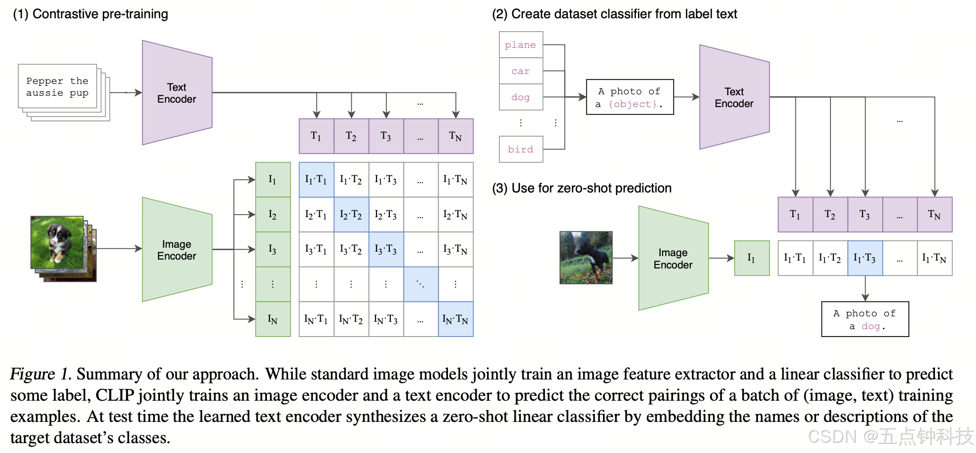
Given a batch of N (image, text) pairs, CLIP is trained to predict which of the N×N possible (image, text) pairings across a batch actually occurred. To do this, CLIP learns a multi-modal embedding space by jointly training an image encoder and text encoder to maximize the cosine similarity of the image and text embeddings of the N real pairs in the batch while minimizing the cosine similarity of the embeddings of the N²-N incorrect pairings. We optimize a symmetric cross entropy loss over these similarity scores.
逐句解读
这是 CLIP 训练目标的精确数学定义:
- Batch 中有 N 对图文。
- N×N 的相似度矩阵:N 个图像向量 × N 个文本向量,共 N² 对。
- 对角线上的 N 个是真实配对(正样本),其余 N²-N 个是负样本。
- 目标:最大化对角线相似度,最小化非对角线相似度。
- “Symmetric cross entropy”:对每一行(图像视角)做 softmax 分类,对每一列(文本视角)做 softmax 分类,两个方向的 loss 取平均。
这个损失函数在 NLP 中被称为 InfoNCE(信息噪声对比估计)。用批内的其他样本作为负样本,batch size 越大,负样本越多,训练越有效——这解释了为什么 CLIP 要用 batch size = 32,768。
3. Section 2.1: Natural Language Supervision
原文
At the core of our approach is the idea of learning perception from supervision contained in natural language. Although early work wrestled with the complexity of natural language when using topic model and n-gram representations, improvements in deep contextual representation learning suggest we now have the tools to effectively leverage this abundant source of supervision.
Learning from natural language has several potential strengths over other training methods. It’s much easier to scale natural language supervision compared to standard crowd-sourced labeling for image classification since it does not require annotations to be in a classic “machine learning compatible format” such as the canonical 1-of-N majority vote “gold label”. Instead, methods which work on natural language can learn passively from the supervision contained in the vast amount of text on the internet. Learning from natural language also has an important advantage over most unsupervised or self-supervised learning approaches in that it doesn’t “just” learn a representation but also connects that representation to language which enables flexible zero-shot transfer.
逐句解读
为什么自然语言监督比其他方式好?
对比人工标注:ImageNet 的标注需要人类工人看图打标签,每张图都要人工决策。自然语言监督不需要——网上的图片本来就有人写的标题、描述、评论,这是被动收集的监督信号,不需要额外的人工劳动。
对比无监督/自监督学习(如 MoCo, SimCLR):这些方法确实能学到很好的视觉表示,但它们的表示是"匿名的"——模型知道这两张图很相似,但不知道"这是一只猫"。CLIP 的表示绑定了语言,所以可以做零样本迁移:你用文字告诉模型新概念,模型立刻就能用。
关键洞察:自然语言监督 = 表示学习 + 语义绑定,一举两得。
4. Section 2.2: Creating a Large Dataset
原文
Existing work has mainly used three datasets, MS-COCO, Visual Genome, and YFCC100M. While MS-COCO and Visual Genome are high quality crowd-labeled datasets, they are small by modern standards with approximately 100,000 training photos each. YFCC100M, at 100 million photos, is a possible alternative, but the metadata for each image is sparse and of varying quality. After filtering to keep only images with natural language titles and/or descriptions in English, the dataset shrunk by a factor of 6 to only 15 million photos.
To address this, we constructed a new dataset of 400 million (image, text) pairs collected from a variety of publicly available sources on the Internet. To attempt to cover as broad a set of visual concepts as possible, we search for (image, text) pairs as part of the construction process whose text includes one of a set of 500,000 queries. We approximately class balance the results by including up to 20,000 (image, text) pairs per query. The resulting dataset has a similar total word count as the WebText dataset used to train GPT-2. We refer to this dataset as WIT for WebImageText.
逐句解读
现有数据集的问题:
| 数据集 | 规模 | 问题 |
|---|---|---|
| MS-COCO | ~10万 | 太小 |
| Visual Genome | ~10万 | 太小 |
| YFCC100M | 1亿(过滤后1500万) | 过滤后太小,元数据质量差 |
WIT 数据集的构建策略:
- 500,000 个查询词:覆盖尽量广的视觉概念(Wikipedia 高频词 + 高 PMI 二元组 + Wikipedia 文章标题 + WordNet 同义词集)
- 每个查询最多 20,000 对:防止某些热门概念(如"猫"“狗”)主导训练数据,实现类平衡
- 总规模:4 亿对,与 GPT-2 训练的 WebText 数据集词数相当
为什么类平衡重要?如果不平衡,模型会过度关注常见概念(如"猫"),忽略稀有但重要的概念(如"扳手"),导致对罕见类别的零样本性能很差。
5. Section 2.3: Pre-Training Method
原文
Due to the large size of our pre-training dataset, over-fitting is not a major concern and the details of training CLIP are simplified compared to the implementation of ConVIRT. We train CLIP from scratch without initializing the image encoder with ImageNet weights or the text encoder with pre-trained weights. We do not use the non-linear projection between the representation and the contrastive embedding space, a change which was introduced by Bachman (2019) and popularized by SimCLR. We instead use only a linear projection to map from each encoder’s representation to the multi-modal embedding space. We did not notice a difference in training efficiency between the two versions and speculate that non-linear projections may be co-adapted with details of current image only in self-supervised representation learning methods. We also simplify the image transformation function. A random square crop from resized images is the only data augmentation used during training. Finally, the temperature parameter τ, is directly optimized during training as a log-parameterized multiplicative scalar to avoid tuning as a hyper-parameter.
逐句解读
这段描述了 CLIP 相比 ConVIRT(其前身)的六个简化:
简化 1:从零训练
- 不用 ImageNet 预训练权重初始化图像编码器
- 不用 GPT-2 权重初始化文本编码器
- 原因:4 亿数据够大,不需要热启动,从零训练也能收敛
简化 2:线性投影代替非线性投影
- SimCLR 发现在图像自监督中,在 encoder 输出后加一个 MLP(非线性投影头)能显著提升性能
- CLIP 只用线性投影,效果相同
- 作者的解释:非线性投影头可能是自监督方法的特有 trick,与对比语言-图像学习的机制不同
简化 3:极简数据增强
- 只用随机裁剪(random square crop from resized image)
- SimCLR 等方法需要大量数据增强(颜色抖动、Gaussian blur、水平翻转等)来防止捷径学习
- CLIP 不需要,因为两个 modality(图像 vs 文字)天然就是非常强的"增强"——它们之间的差异足够大,模型不会走捷径
简化 4:温度参数 τ 可学习
- 其他方法把 τ 当超参数手动调
- CLIP 把 log(τ) 作为可学习参数,让模型自己决定置信度范围
- 用 log-parameterize(即 τ = exp(log_τ))的原因:保证 τ 永远为正,数值稳定
InfoNCE Loss 数学形式
对于 batch 中第 i 张图像,其损失为:
L_image_i = -log( exp(sim(I_i, T_i)/τ) / Σ_j exp(sim(I_i, T_j)/τ) )
对称损失:
L_text_i = -log( exp(sim(T_i, I_i)/τ) / Σ_j exp(sim(T_j, I_i)/τ) )
总损失:
L = (1/N) Σ_i (L_image_i + L_text_i) / 2
其中 sim(u, v) = u·v / (‖u‖·‖v‖)(余弦相似度),N 是 batch size,τ 是可学习温度。
6. Section 2.4: Model Architecture
原文
We consider two different architectures for the image encoder. For the first, we use ResNet-50 as the base architecture for the image encoder due to its widespread adoption and proven performance. We make several modifications to the original version using the ResNet-D improvements from He et al. (2019) and the antialiased rect-2 blur pooling from Zhang (2019). We also replace the global average pooling layer with an attention pooling mechanism. The attention pooling is implemented as a single layer of “transformer-style” multi-head QKV attention where the query is conditioned on the global average-pooled representation of the image.
For the second architecture, we experiment with the recently introduced Vision Transformer (ViT). We closely follow their implementation with only the minor modification of adding an additional layer normalization to the combined patch and position embeddings before the transformer and use a slightly different initialization scheme.
The text encoder is a Transformer with the architecture modifications described in GPT-2. As a base size we use a 63M-parameter 12-layer 512-wide model with 8 attention heads. The transformer operates on a lower-cased byte pair encoding (BPE) representation of the text with a 49,152 vocab size. For computational efficiency, the max sequence length was capped at 76. The text sequence is bracketed with [SOS] and [EOS] tokens and the activations of the highest layer of the transformer at the [EOS] token are treated as the feature representation of the text which is layer normalized and then linearly projected into the multi-modal embedding space. Masked self-attention was used in the text encoder to preserve the ability to initialize with a pre-trained language model or add language modeling as an auxiliary objective.
逐句解读
图像编码器选项一:改进版 ResNet
原始 ResNet-50 的三处改进:
- ResNet-D 改进:把步长为 2 的第一个 1×1 卷积改为先做平均池化再 1×1 卷积,解决信息丢失问题
- Antialiased blur pooling:在下采样之前加高斯模糊,减少 aliasing 现象,提升平移等变性
- Attention pooling 代替 Global Average Pooling:最后不再对所有空间位置平均,而是用 Transformer 风格的 QKV 注意力聚合——query 是全局平均池化的结果,key/value 是每个空间位置的特征。这让模型能"关注"最重要的区域。
图像编码器选项二:ViT
几乎原版 ViT,只有两个细微修改:
- 在 patch embedding + position embedding 后额外加一个 LayerNorm(Pre-LN 风格,稳定训练)
- 稍微不同的权重初始化方案
文本编码器:GPT-2 风格 Transformer
关键参数(基础版):
- 12 层 Transformer
- 隐藏维度 512
- 8 个注意力头
- 词汇表大小 49,152(BPE)
- 最大序列长度 76(加 [SOS] 和 [EOS] = 78)
重要设计:取 [EOS] 位置的输出(而不是 [CLS])
- GPT-2 使用因果(单向)注意力掩码,[EOS] 是序列最后一个 token,它的表示能"看到"整个序列的所有信息
- LayerNorm → 线性投影 → 多模态嵌入空间
为什么用因果注意力?
论文说"保留用预训练语言模型初始化或加入语言建模辅助目标的能力"——虽然最终没这么做,但设计上留了余地。对于 VLA 研究者:这意味着 CLIP 的文本编码器天然兼容 autoregressive LLM,是后来 LLaVA、InstructBLIP 等模型的重要桥梁。
7. Section 2.5: Training
原文
We train a series of 5 ResNets and 3 Vision Transformers. For the ResNets we train a ResNet-50, a ResNet-101, and then 3 more which follow EfficientNet-style model scaling and use approximately 4x, 16x, and 64x the compute of a ResNet-50. We train all models for 32 epochs. We use the Adam optimizer with decoupled weight decay regularization applied to all weights that are not gains or biases, and decay the learning rate using a cosine schedule. The learnable temperature parameter τ was initialized to the equivalent of 0.07 and clipped to prevent scaling the logits by more than 100 which we found necessary to prevent training instability. We use a very large minibatch size of 32,768. Mixed-precision was used to accelerate training and save memory. The largest ResNet model, RN50x64, took 18 days to train on 592 V100 GPUs while the largest Vision Transformer took 12 days on 256 V100 GPUs.
逐句解读
训练配置总览:
| 参数 | 值 |
|---|---|
| 训练 epoch | 32 |
| Batch size | 32,768(极大) |
| 优化器 | AdamW(Adam + decoupled weight decay) |
| 学习率调度 | Cosine 退火 |
| 温度初始值 | τ = 0.07(即 1/0.07 ≈ 14.3 的缩放) |
| 温度上限 | τ 的最小值限制使得 logit 缩放 ≤ 100 |
| 精度 | 混合精度(FP16 + FP32) |
为什么 batch size = 32,768?
InfoNCE Loss 需要大量负样本。Batch size 越大:
- 每个正样本对应的负样本越多(32,767 个)
- 负样本分布更广,更能代表真实的"困难负样本"
- 理论上相当于用更大的"动态字典"做对比学习
代价:显存需求极大。解决方案:梯度检查点(gradient checkpointing)+ 半精度 Adam 统计量 + 相似度计算分片(每块 GPU 只算自己 local batch 的那部分相似度矩阵)
ViT 比 ResNet 计算更高效:最大 ViT 模型(ViT-L/14)在 256 块 V100 上只需 12 天,而最大 ResNet(RN50x64)在 592 块 V100 上需要 18 天。这印证了 ViT 在大数据上更高效的结论。
8. Section 3.1: Zero-Shot Transfer
原文
CLIP is pre-trained to predict if an image and a text snippet are paired together in its dataset. To perform zero-shot classification, we reuse this capability. For each dataset, we use the names of all the classes in the dataset as the set of potential text pairings and predict the most probable (image, text) pair according to CLIP. We first compute the feature embedding of the image and the feature embedding of the set of possible texts by their respective encoders. The cosine similarity of these embeddings is then calculated, scaled by a temperature parameter τ, and normalized into a probability distribution via a softmax.
Note that this prediction layer is a multinomial logistic regression classifier with L2-normalized inputs, L2-normalized weights, no bias, and temperature scaling. When interpreted this way, the image encoder is the computer vision backbone which computes a feature representation for the image and the text encoder is a hypernetwork which generates the weights of a linear classifier based on the text specifying the visual concepts that the classes represent.
逐句解读
零样本分类的完整流程:
输入:一张图像 + K 个类别名(文字)

步骤1:文本编码
  for i in range(K):
      text_i = "A photo of a {class_name_i}."
      w_i = text_encoder(text_i)  # 形状:(embed_dim,)
      w_i = normalize(w_i)  # L2 归一化

步骤2:图像编码
  v = image_encoder(image)  # 形状:(embed_dim,)
  v = normalize(v)  # L2 归一化

步骤3:计算 logits
  logits[i] = τ⁻¹ * dot(v, w_i)  # 余弦相似度 * 温度倒数

步骤4:预测
  prediction = argmax(softmax(logits))
“文本编码器是超网络(hypernetwork)” 这个比喻非常深刻:
- 普通分类器:有固定的权重矩阵 W ∈ R^(K×d),只能分 K 个预先确定的类别
- CLIP:文本编码器动态生成 W 的每一行——你给什么文字描述,它就生成对应那一行权重
- 这意味着:类别数量不受限制,类别描述可以随时更换,迁移到新任务不需要任何梯度更新
9. Section 3.2: Prompt Engineering
原文
A common issue is polysemy. When the name of a class is the only information provided to CLIP’s text encoder it is unable to differentiate which word sense is meant due to the lack of context. In some cases multiple meanings of the same word might be included as different classes in the same dataset! This happens in ImageNet which contains both construction cranes and cranes that fly.
We found that using the prompt template “A photo of a {label}.” to be a good default that helps specify the text is about the content of the image. This often improves performance over the baseline of using only the label text. For instance, just using this prompt improves accuracy on ImageNet by 1.3%.
We also experimented with ensembling over multiple zero-shot classifiers. We construct the ensemble over the embedding space instead of probability space. This allows us to cache a single set of averaged text embeddings so that the compute cost of the ensemble is the same as using a single classifier when amortized over many predictions. On ImageNet, we ensemble 80 different context prompts and this improves performance by an additional 3.5% over the single default prompt. When considered together, prompt engineering and ensembling improve ImageNet accuracy by almost 5%.
逐句解读
问题 1:多义词(Polysemy)
ImageNet 里有"crane"(建筑吊车)和"crane"(鹤)两个类别。如果你把裸词"crane"送给文本编码器,它不知道是哪个意思。加上上下文"A photo of a crane."也不够——还是两个都符合。需要更精确的模板如"A photo of a crane bird."才能消歧。
问题 2:训练分布偏移
CLIP 的预训练文本通常是完整句子(如"A cute cat sitting on a windowsill"),而下游数据集只给你一个词(“cat”)。这造成了分布偏移,用"A photo of a {label}."这样的模板来缩小这个 gap。
Ensemble 的技巧:
- 不是在概率空间做集成(会需要多次推理),而是在嵌入空间对多个文本模板的嵌入向量取平均后归一化
- 一次性缓存所有类别的平均嵌入,推理时计算开销与单模板完全相同
- 80 路集成 + 工程化模板 → ImageNet 零样本 +5%
对 VLA 研究的启示:在机器人任务中,任务描述的措辞会极大影响 CLIP-based VLA 的性能。"pick up the red cup"和"grab the cup on the left"指向同一动作,但对模型来说差异很大。这是 VLA 工程中需要注意的点。
10. Section 3.4: Robustness
原文
All zero-shot CLIP models improve effective robustness by a large amount and reduce the size of the gap between ImageNet accuracy and accuracy under distribution shift by up to 75%.
Although adapting CLIP to the ImageNet distribution increases its ImageNet accuracy by 9.2% to 85.4% overall, average accuracy under distribution shift slightly decreases.
It is surprising to see a 9.2% increase in accuracy, which corresponds to roughly 3 years of improvement in SOTA, fail to translate into any improvement in average performance under distribution shift.
逐句解读
分布偏移实验的核心发现:
发现 1:零样本 CLIP 对分布偏移的鲁棒性极强
零样本 CLIP 把"ImageNet 精度 vs 分布偏移精度"之间的差距缩小了 75%。原因:零样本模型没有针对 ImageNet 的分布拟合,不会学到 ImageNet 特有的虚假相关性(spurious correlations)。
发现 2:监督微调虽然提升 ImageNet 精度,但损害鲁棒性
把 CLIP 在 ImageNet 上做线性探测(logistic regression):
- ImageNet 精度:+9.2%(相当于 3 年的 SOTA 进展)
- 分布偏移下的精度:下降
这是一个令人震惊的结论:为特定数据集优化越多,对其他分布的泛化越差。这不是因为 CLIP 特殊,而是监督学习的普遍问题。
对 VLA 研究的深刻启示:
在水下环境部署视觉模型时,这个结论极为重要。在某个特定水下场景微调的 VLA,很可能在稍微不同的光线/水质/能见度条件下快速退化。基于 CLIP 的零样本策略比完全微调的策略往往有更好的跨域鲁棒性。
11. Section 4: Human Comparison
原文
Interestingly, humans went from a performance average of 54% to 76% with just one training example per class, and the marginal gain from an additional training example is minimal. The gain in accuracy going from zero to one shot is almost entirely on images that humans were uncertain about. This suggests that humans “know what they don’t know” and are able to update their priors on the images they are most uncertain in based on a single example.
Given this, it seems that while CLIP is a promising training strategy for zero-shot performance and does well on tests of natural distribution shift, there is a large difference between how humans learn from a few examples and the few-shot methods in this paper.
逐句解读
人类 vs CLIP 对比(Oxford Pets 数据集,37 类猫狗品种):
| 模型/人类 | 精度 |
|---|---|
| 零样本人类 | 54% |
| 零样本 CLIP | 93.5% |
| 一样本人类 | 76% |
| 两样本人类 | 76% |
CLIP 零样本完胜人类两样本。但这并不说明 CLIP"比人聪明"——因为 CLIP 的训练数据中可能包含这些品种的大量信息,而零样本的人类真的完全不认识这些冷门犬种。
人类少样本学习的机制:人知道自己不确定的地方,能用一个样本精准更新不确定的判断。CLIP 的 few-shot(线性探测)方法则是暴力地用监督信号调整所有类的边界,效率远低于人类。
这说明的局限:CLIP 不是在"理解"图片,而是在做统计匹配。真正的视觉理解需要能从极少样本中快速学习新概念的能力,这是未来研究(如 meta-learning 与 VLA 结合)的方向。
12. Section 5: Limitations
原文(论文 Section 7,Limitations)
CLIP still falls far short of state-of-the-art task-specific models on several tasks. The best CLIP model is roughly equivalent to the performance of a ResNet-50 on ImageNet, which is not a state of the art model. There is still plenty of room to improve zero-shot performance. CLIP is also limited by its training set — any bias present in the 400 million pairs will be reflected in the model. Further, CLIP applies a learned linear projection to map from each encoder’s representation to the contrastive embedding space, which may limit expressiveness. CLIP has poor performance on some tasks, such as counting objects, abstract reasoning, and fine-grained classification of highly specialized images such as satellite imagery or medical scans. Finally, out-of-distribution data can still hurt CLIP.
逐句解读
局限 1:零样本精度仍有差距
零样本 CLIP ≈ ResNet-50 全监督(ImageNet 76.2%),但最先进的监督模型早已超过 90%。CLIP 的零样本能力虽令人印象深刻,但距"全面替代监督学习"还很远。
局限 2:数据集偏见
WIT 来自互联网,互联网文本有性别、种族、地域等方面的偏见。这些偏见直接编码进了模型的表示空间。
局限 3:特定任务弱项
- 计数(如"图中有几个苹果?"):CLIP 没有显式的计数能力
- 抽象推理:CLIP 做的是语义匹配,不是逻辑推理
- 专业领域:卫星图像、医学影像——这类图像在 WIT 中极少,CLIP 对它们的理解很浅
对 UUV VLA 研究的直接影响:水下图像是典型的"专业领域稀缺数据"场景。CLIP 在水下场景的直接迁移能力会受限,可能需要专门的水下图文预训练数据(如通过爬取水下机器人论文、海洋生物学文献等方式构建)。
13. CLIP 网络结构完整源码解析
以下基于 OpenAI 官方实现
clip/model.py(https://github.com/openai/CLIP)进行完整解析,包含每一层的输入/输出维度。
13.1 整体架构概览
CLIP 模型
├── 视觉编码器(二选一)
│   ├── ModifiedResNet(ResNet-50/101/50×4/50×16/50×64)
│   └── VisionTransformer(ViT-B/32, ViT-B/16, ViT-L/14)
├── 文本编码器
│   └── Transformer(GPT-2 风格)
├── 图像投影矩阵(线性层)
├── 文本投影矩阵(线性层)
└── 可学习温度参数 log_scale
CLIP 主类初始化参数:
class CLIP(nn.Module):
    def __init__(
        self,
        embed_dim: int,           # 多模态嵌入空间维度,如 512
        # 视觉参数
        image_resolution: int,    # 输入图像分辨率,如 224
        vision_layers: Union[Tuple[int,int,int,int], int],
                                  # ResNet → tuple(3,4,6,3); ViT → int(如12)
        vision_width: int,        # 视觉编码器宽度,如 64(ResNet) 或 768(ViT)
        vision_patch_size: int,   # ViT 的 patch 大小,如 16 或 32
        # 文本参数
        context_length: int,      # 最大序列长度,76
        vocab_size: int,          # 词表大小,49152
        transformer_width: int,   # Transformer 隐藏维度,512
        transformer_heads: int,   # 注意力头数,8
        transformer_layers: int,  # Transformer 层数,12
    )
模型选择逻辑:
if isinstance(vision_layers, (tuple, list)):
    # vision_layers 是 tuple → 使用 ModifiedResNet
    vision_heads = vision_width * 32 // 64
    # ResNet-50: vision_width=64, vision_heads = 64*32//64 = 32
    self.visual = ModifiedResNet(...)
else:
    # vision_layers 是 int → 使用 VisionTransformer
    vision_heads = vision_width // 64
    # ViT-B/16: vision_width=768, vision_heads = 768//64 = 12
    self.visual = VisionTransformer(...)
各模型规格对照表:
| 模型 | 图像编码器类型 | image_resolution | vision_width | vision_layers | embed_dim |
|---|---|---|---|---|---|
| RN50 | ModifiedResNet | 224 | 64 | (3,4,6,3) | 1024 |
| RN101 | ModifiedResNet | 224 | 64 | (3,4,23,3) | 512 |
| RN50×4 | ModifiedResNet | 288 | 80 | (4,5,7,4) | 640 |
| RN50×16 | ModifiedResNet | 384 | 96 | (6,8,18,8) | 768 |
| RN50×64 | ModifiedResNet | 448 | 128 | (3,15,36,10) | 1024 |
| ViT-B/32 | VisionTransformer | 224 | 768 | 12 | 512 |
| ViT-B/16 | VisionTransformer | 224 | 768 | 12 | 512 |
| ViT-L/14 | VisionTransformer | 224 | 1024 | 24 | 768 |
| ViT-L/14@336 | VisionTransformer | 336 | 1024 | 24 | 768 |
13.2 ModifiedResNet 逐层解析
以 RN50(vision_width=64, layers=(3,4,6,3), output_dim=1024)为例:
class ModifiedResNet(nn.Module):
    def __init__(self, layers, output_dim, heads, input_resolution=224, width=64):
阶段 0:Stem(主干入口)
# 三个 3×3 卷积代替原 ResNet 的单个 7×7 卷积(ResNet-D 改进)
self.conv1 = nn.Conv2d(3, width//2, kernel_size=3, stride=2, padding=1, bias=False)
self.bn1   = nn.BatchNorm2d(width//2)
self.relu1 = nn.ReLU(inplace=True)
# width//2 = 32

self.conv2 = nn.Conv2d(width//2, width//2, kernel_size=3, padding=1, bias=False)
self.bn2   = nn.BatchNorm2d(width//2)
self.relu2 = nn.ReLU(inplace=True)

self.conv3 = nn.Conv2d(width//2, width, kernel_size=3, padding=1, bias=False)
self.bn3   = nn.BatchNorm2d(width)
self.relu3 = nn.ReLU(inplace=True)
# width = 64

self.avgpool = nn.AvgPool2d(2)  # antialiased blur pooling
维度变化:
输入:(B, 3, 224, 224)
→ conv1(stride=2) → (B, 32, 112, 112)
→ conv2           → (B, 32, 112, 112)
→ conv3           → (B, 64, 112, 112)
→ avgpool(2)      → (B, 64, 56, 56)
阶段 1-4:ResNet Blocks
# layer1: width=64,  stride=1, blocks=3
self.layer1 = self._make_layer(width,      layers[0])
# layer2: width=128, stride=2, blocks=4
self.layer2 = self._make_layer(width*2,    layers[1], stride=2)
# layer3: width=256, stride=2, blocks=6
self.layer3 = self._make_layer(width*4,    layers[2], stride=2)
# layer4: width=512, stride=2, blocks=3
self.layer4 = self._make_layer(width*8,    layers[3], stride=2)
Bottleneck block(每个 block 的内部结构):
class Bottleneck(nn.Module):
    expansion = 4
    def forward(self, x):
        # x: (B, C_in, H, W)
        out = self.relu(self.bn1(self.conv1(x)))  # 1×1 降维
        out = self.relu(self.bn2(self.conv2(out))) # 3×3 卷积
        out = self.bn3(self.conv3(out))            # 1×1 升维 (×4)
        if self.downsample:
            x = self.downsample(x)
        return self.relu(out + x)
完整维度变化(RN50):
Stem 输出:  (B, 64, 56, 56)

Layer1 (3 blocks, stride=1):
  → Bottleneck: 64 → 64 → 256
  → (B, 256, 56, 56)

Layer2 (4 blocks, stride=2):
  → Bottleneck: 256 → 128 → 512
  → (B, 512, 28, 28)

Layer3 (6 blocks, stride=2):
  → Bottleneck: 512 → 256 → 1024
  → (B, 1024, 14, 14)

Layer4 (3 blocks, stride=2):
  → Bottleneck: 1024 → 512 → 2048
  → (B, 2048, 7, 7)
阶段 5:Attention Pooling(代替 Global Average Pooling)
embed_dim = width * 32  # = 64 * 32 = 2048(feature dim)
self.attnpool = AttentionPool2d(
    spacial_dim    = input_resolution // 32,  # 224//32 = 7
    embed_dim      = embed_dim,               # 2048
    num_heads      = heads,                   # 32
    output_dim     = output_dim               # 1024 (embed_dim of CLIP)
)
AttentionPool2d 内部:
class AttentionPool2d(nn.Module):
    def __init__(self, spacial_dim, embed_dim, num_heads, output_dim=None):
        super().__init__()
        # 位置嵌入:49个空间位置 + 1个全局query,每个embed_dim维
        self.positional_embedding = nn.Parameter(
            torch.randn(spacial_dim**2 + 1, embed_dim) / embed_dim**0.5
        )
        # QKV 投影
        self.k_proj = nn.Linear(embed_dim, embed_dim)
        self.q_proj = nn.Linear(embed_dim, embed_dim)
        self.v_proj = nn.Linear(embed_dim, embed_dim)
        # 输出投影
        self.c_proj = nn.Linear(embed_dim, output_dim or embed_dim)
        self.num_heads = num_heads

    def forward(self, x):
        # x: (B, C, H, W) = (B, 2048, 7, 7)
        x = x.flatten(start_dim=2).permute(2, 0, 1)
        # → (HW, B, C) = (49, B, 2048)

        # 全局平均池化作为 query
        x = torch.cat([x.mean(dim=0, keepdim=True), x], dim=0)
        # → (50, B, 2048)  [第0位是global query, 1-49是各空间位置]

        # 加位置嵌入
        x = x + self.positional_embedding[:, None, :].to(x.dtype)

        # 多头注意力(query=第0位,key/value=全部50位)
        x, _ = F.multi_head_attention_forward(
            query=x[:1],       # (1, B, 2048) — 只用 global query
            key=x,             # (50, B, 2048)
            value=x,           # (50, B, 2048)
            ...
        )
        # → (1, B, 2048)
        x = x.squeeze(0)      # (B, 2048)
        x = self.c_proj(x)    # 线性投影
        # → (B, 1024)  = (B, output_dim)
        return x
完整维度总结(ModifiedResNet RN50):
输入:              (B, 3, 224, 224)
Stem:              (B, 64, 56, 56)
Layer1:            (B, 256, 56, 56)
Layer2:            (B, 512, 28, 28)
Layer3:            (B, 1024, 14, 14)
Layer4:            (B, 2048, 7, 7)
AttentionPool:     (B, 1024)          ← 图像特征(投影前)
image_projection:  (B, 512)           ← 图像嵌入(投影后)
L2-normalize:      (B, 512)
注:RN50 的
output_dim=1024,embed_dim=512,所以 AttentionPool 输出 1024,再经图像投影 (1024→512) 得到最终嵌入。
13.3 VisionTransformer 逐层解析
以 ViT-B/16(vision_width=768, vision_layers=12, patch_size=16, image_resolution=224)为例:
class VisionTransformer(nn.Module):
    def __init__(self, input_resolution, patch_size, width, layers, heads, output_dim):
        # input_resolution=224, patch_size=16, width=768
        # layers=12, heads=12, output_dim=512

        self.input_resolution = input_resolution
        self.output_dim = output_dim

        # Patch embedding
        self.conv1 = nn.Conv2d(
            in_channels=3,
            out_channels=width,       # 768
            kernel_size=patch_size,   # 16
            stride=patch_size,        # 16(无重叠分割)
            bias=False
        )

        scale = width ** -0.5  # 1/sqrt(768) ≈ 0.036

        # Class token([CLS] token)
        self.class_embedding = nn.Parameter(scale * torch.randn(width))
        # shape: (768,)

        # 位置嵌入((H/P)*(W/P) + 1 个位置)
        self.positional_embedding = nn.Parameter(
            scale * torch.randn((input_resolution // patch_size) ** 2 + 1, width)
        )
        # shape: (14*14+1, 768) = (197, 768)

        # Pre-Transformer LayerNorm(CLIP 特有,ViT 原版没有)
        self.ln_pre = nn.LayerNorm(width)

        # Transformer 主体
        self.transformer = Transformer(width, layers, heads)

        # Post-Transformer LayerNorm
        self.ln_post = nn.LayerNorm(width)

        # 投影矩阵
        self.proj = nn.Parameter(scale * torch.randn(width, output_dim))
        # shape: (768, 512)
前向传播:
def forward(self, x: torch.Tensor):
    # x: (B, 3, 224, 224)

    # Step 1: Patch Embedding
    x = self.conv1(x)
    # → (B, 768, 14, 14)  [224/16=14, 14×14=196 patches]

    x = x.reshape(x.shape[0], x.shape[1], -1)
    # → (B, 768, 196)

    x = x.permute(0, 2, 1)
    # → (B, 196, 768)

    # Step 2: 拼接 Class Token
    # class_embedding: (768,) → (1, 1, 768) → (B, 1, 768)
    x = torch.cat([
        self.class_embedding.to(x.dtype) + torch.zeros(x.shape[0], 1, x.shape[-1]),
        x
    ], dim=1)
    # → (B, 197, 768)  [第0位是[CLS], 1-196是各 patch]

    # Step 3: 加位置嵌入
    x = x + self.positional_embedding.to(x.dtype)
    # positional_embedding: (197, 768) → 广播到 (B, 197, 768)
    # → (B, 197, 768)

    # Step 4: Pre-LN(CLIP 特有)
    x = self.ln_pre(x)
    # → (B, 197, 768)

    # Step 5: Transformer
    x = x.permute(1, 0, 2)  # NLD → LND
    # → (197, B, 768)
    x = self.transformer(x)
    # → (197, B, 768)
    x = x.permute(1, 0, 2)  # LND → NLD
    # → (B, 197, 768)

    # Step 6: 取 [CLS] token(第0位)
    x = self.ln_post(x[:, 0, :])
    # → (B, 768)

    # Step 7: 线性投影
    if self.proj is not None:
        x = x @ self.proj
        # (B, 768) @ (768, 512) = (B, 512)

    return x  # (B, 512)
完整维度总结(ViT-B/16):
输入:                    (B, 3, 224, 224)
Conv1 (patch embed):     (B, 768, 14, 14)
Reshape + Permute:       (B, 196, 768)
+CLS token:              (B, 197, 768)
+Position Embedding:     (B, 197, 768)
Pre-LN:                  (B, 197, 768)
Permute (NLD→LND):       (197, B, 768)
Transformer (12 layers): (197, B, 768)
Permute (LND→NLD):       (B, 197, 768)
取 CLS token + Post-LN:  (B, 768)
线性投影 (768→512):       (B, 512)          ← 图像特征
L2-normalize:            (B, 512)
13.4 Transformer 逐层解析(Transformer Block)
以文本编码器基础版(width=512, layers=12, heads=8)为例:
class ResidualAttentionBlock(nn.Module):
    def __init__(self, d_model: int, n_head: int, attn_mask: torch.Tensor = None):
        super().__init__()
        # Multi-Head Self-Attention
        self.attn = nn.MultiheadAttention(d_model, n_head)
        # Layer Norms(Pre-LN 结构)
        self.ln_1 = nn.LayerNorm(d_model)
        # MLP: d_model → 4*d_model → d_model
        self.mlp = nn.Sequential(
            nn.Linear(d_model, d_model * 4),
            QuickGELU(),
            nn.Linear(d_model * 4, d_model)
        )
        self.ln_2 = nn.LayerNorm(d_model)
        self.attn_mask = attn_mask

    def attention(self, x: torch.Tensor):
        # x: (L, B, d_model)
        self.attn_mask = self.attn_mask.to(dtype=x.dtype, device=x.device) \
                         if self.attn_mask is not None else None
        return self.attn(x, x, x, need_weights=False, attn_mask=self.attn_mask)[0]

    def forward(self, x: torch.Tensor):
        # Pre-LN + Self-Attention + Residual
        x = x + self.attention(self.ln_1(x))
        # Pre-LN + MLP + Residual
        x = x + self.mlp(self.ln_2(x))
        return x
单个 Transformer Block 的维度流动(以文本编码器为例):
输入 x:           (L, B, 512)    [L=76+2=78, 序列长度]

--- Attention Sub-block ---
LN-1(x):          (L, B, 512)
MHSA:
  Q = W_q @ x:  (L, B, 512) → split → (L, B, 8, 64) [8 heads, 64 dim each]
  K = W_k @ x:  同上
  V = W_v @ x:  同上
  Attention:    QK^T/√64 + mask → softmax → @V → (L, B, 8, 64)
  Concat:       (L, B, 512)
  W_out @ ...:  (L, B, 512)
Residual:         (L, B, 512)

--- FFN Sub-block ---
LN-2(x):          (L, B, 512)
Linear(512→2048): (L, B, 2048)
QuickGELU:        (L, B, 2048)
Linear(2048→512): (L, B, 512)
Residual:         (L, B, 512)

输出:             (L, B, 512)
13.5 文本编码器逐层解析
class CLIP(nn.Module):
    def encode_text(self, text):
        # text: (B, context_length) = (B, 77)
        # 每个元素是 token id,范围 [0, vocab_size)

        # Step 1: Token Embedding
        x = self.token_embedding(text).type(self.dtype)
        # token_embedding: (vocab_size, transformer_width) = (49152, 512)
        # → (B, 77, 512)

        # Step 2: 加位置嵌入
        x = x + self.positional_embedding.type(self.dtype)
        # positional_embedding: (context_length, transformer_width) = (77, 512)
        # → (B, 77, 512)

        # Step 3: Transformer
        x = x.permute(1, 0, 2)   # NLD → LND
        # → (77, B, 512)
        x = self.transformer(x)
        # 12层 Transformer Block,带因果掩码
        # → (77, B, 512)
        x = x.permute(1, 0, 2)   # LND → NLD
        # → (B, 77, 512)

        # Step 4: 取 [EOS] token 位置
        # argmax(text) 给出每个样本中值最大的 token 位置,
        # 在 BPE 中 [EOS] token 有最大的 token id
        x = self.ln_final(x).type(self.dtype)
        # → (B, 77, 512)
        x = x[torch.arange(x.shape[0]), text.argmax(dim=-1)]
        # → (B, 512)  [取每个样本的 EOS 位置]

        # Step 5: 线性投影
        x = x @ self.text_projection
        # text_projection: (transformer_width, embed_dim) = (512, 512)
        # → (B, 512)

        return x  # (B, 512)
完整维度总结(文本编码器,基础版):
输入 token ids:         (B, 77)       [BPE token ids, [SOS] ... [EOS]]
Token Embedding:        (B, 77, 512)
+Positional Embedding:  (B, 77, 512)
Permute (NLD→LND):      (77, B, 512)
Transformer (12层):     (77, B, 512)  [每层: 512→2048→512 MLP + 8-head MHSA]
Permute (LND→NLD):      (B, 77, 512)
LN-Final:               (B, 77, 512)
取 EOS 位置:            (B, 512)
线性投影 (512→512):      (B, 512)      ← 文本特征
L2-normalize:           (B, 512)
注意:文本使用因果注意力掩码(causal/autoregressive mask),即每个位置只能 attend 到它之前的位置。这和 GPT-2 一致,但和 BERT 的双向注意力不同。
13.6 前向传播与对比损失
class CLIP(nn.Module):
    def forward(self, image, text):
        # image: (B, 3, H, W)
        # text:  (B, 77)

        # Step 1: 编码
        image_features = self.encode_image(image)  # (B, embed_dim)
        text_features  = self.encode_text(text)    # (B, embed_dim)

        # Step 2: L2 归一化
        image_features = image_features / image_features.norm(dim=1, keepdim=True)
        text_features  = text_features  / text_features.norm(dim=1, keepdim=True)
        # 归一化后,内积 = 余弦相似度

        # Step 3: 计算相似度矩阵
        logit_scale = self.logit_scale.exp()
        # logit_scale = τ⁻¹(初始化约为 14.3)

        logits_per_image = logit_scale * image_features @ text_features.t()
        # (B, embed_dim) @ (embed_dim, B) = (B, B)
        # logits_per_image[i][j] = τ⁻¹ * cos_sim(image_i, text_j)

        logits_per_text = logits_per_image.t()
        # (B, B)

        return logits_per_image, logits_per_text
        # 对角线是正样本,其余是负样本
训练 Loss 计算(论文 Pseudocode):
def contrastive_loss(logits_per_image, logits_per_text):
    B = logits_per_image.shape[0]
    labels = torch.arange(B)  # [0, 1, 2, ..., B-1]

    # 图像视角:对每行做 softmax,正确答案是对角线(第 i 行的第 i 列)
    loss_i = F.cross_entropy(logits_per_image, labels)

    # 文本视角:对每列做 softmax
    loss_t = F.cross_entropy(logits_per_text, labels)

    # 对称损失取平均
    loss = (loss_i + loss_t) / 2
    return loss
13.7 零样本推理流程(完整代码)
import torch
import clip

# 加载模型
model, preprocess = clip.load("ViT-B/16", device="cuda")

# ============ 零样本分类 ============

# 1. 准备类别文本
class_names = ["cat", "dog", "airplane", "car"]
texts = [f"A photo of a {name}." for name in class_names]
text_tokens = clip.tokenize(texts).cuda()
# → (4, 77)  [4个类别,每个77个token]

# 2. 编码文本(只需一次)
with torch.no_grad():
    text_features = model.encode_text(text_tokens)
    # → (4, 512)
    text_features /= text_features.norm(dim=-1, keepdim=True)
    # → (4, 512),L2归一化

# 3. 对每张图像进行分类
image = preprocess(pil_image).unsqueeze(0).cuda()
# → (1, 3, 224, 224)

with torch.no_grad():
    image_features = model.encode_image(image)
    # → (1, 512)
    image_features /= image_features.norm(dim=-1, keepdim=True)
    # → (1, 512)

    # 4. 计算相似度
    similarity = (100.0 * image_features @ text_features.T).softmax(dim=-1)
    # (1, 512) @ (512, 4) = (1, 4)
    # softmax → (1, 4)  [4个类别的概率]

    values, indices = similarity.topk(1)
    # 最大概率对应的类别即为预测结果
    print(f"预测类别: {class_names[indices[0][0]]}, 概率: {values[0][0]:.4f}")
这里有个小细节要注意,对角线正样本是人为定义的监督信号,不是数据自然属性。代码通过 labels = arange(batch_size) 这个简单的数学约定,把"配对"问题转化成了标准的分类问题。因此,在数据加载器加载数据时,会自动的将配对正确的图文的索引对齐。这是对比学习巧妙之处的精髓!
13.8 维度变化总图
========== ViT-B/16 模型(最常用)完整维度流 ==========

【图像侧】
输入图像:           (B, 3, 224, 224)
       ↓ Conv2d(3→768, 16×16, stride=16)
Patch Embedding:    (B, 768, 14, 14)
       ↓ reshape + permute
Token序列:          (B, 196, 768)
       ↓ concat [CLS]
+CLS:               (B, 197, 768)
       ↓ + positional_embedding(197, 768)
+Pos Embed:         (B, 197, 768)
       ↓ LayerNorm (Pre-LN,CLIP特有)
LN-pre:             (B, 197, 768)
       ↓ permute(1,0,2)
Transformer输入:    (197, B, 768)
       ↓ × 12 Transformer Blocks
         每块: MHSA(12头, 64维/头) + FFN(768→3072→768)
Transformer输出:    (197, B, 768)
       ↓ 取第0位[CLS] + LayerNorm
CLS特征:            (B, 768)
       ↓ @ proj(768, 512)
图像嵌入:           (B, 512)
       ↓ L2归一化
归一化图像嵌入:      (B, 512)

【文本侧】
输入文本:           (B, 77)     [token ids]
       ↓ token_embedding(49152, 512)
Token Embed:        (B, 77, 512)
       ↓ + positional_embedding(77, 512)
+Pos Embed:         (B, 77, 512)
       ↓ permute(1,0,2)
Transformer输入:    (77, B, 512)
       ↓ × 12 Transformer Blocks (带因果掩码)
         每块: MHSA(8头, 64维/头) + FFN(512→2048→512)
Transformer输出:    (77, B, 512)
       ↓ 取[EOS]位置 + LayerNorm
EOS特征:            (B, 512)
       ↓ @ text_projection(512, 512)
文本嵌入:           (B, 512)
       ↓ L2归一化
归一化文本嵌入:      (B, 512)

【相似度计算】
logit_scale × (B,512) @ (512,B) = (B, B) 相似度矩阵
对角线=正样本,非对角线=负样本
↓
对称 Cross-Entropy Loss(InfoNCE)
附录:模型参数量统计
| 组件 | ViT-B/16 | 参数量 |
|---|---|---|
| Patch Embedding | Conv2d(3,768,16,16) | 3×768×16×16 = 589K |
| CLS Token | (768,) | 768 |
| Position Embedding | (197, 768) | 151K |
| Transformer × 12 | MHSA + FFN | ≈85M |
| LN-final | (768,) ×2 | 1.5K |
| Projection | (768, 512) | 393K |
| 图像编码器合计 | ≈86M | |
| Token Embedding | (49152, 512) | 25M |
| Position Embedding | (77, 512) | 39K |
| Transformer × 12 | MHSA + FFN | ≈38M |
| Text Projection | (512, 512) | 262K |
| 文本编码器合计 | ≈63M | |
| 总计 | ≈149M |

有“AI”的1024 = 2048,欢迎大家加入2048 AI社区
更多推荐

 6
6 0
0- 0


 已为社区贡献5条内容

所有评论(0)