【Transformer开山之作】这篇论文如何彻底改变了AI世界？逐段精读《Attention is All You Need》

《Attention Is All You Need》论文摘要： Transformer是一种基于纯注意力机制的序列转换模型，摒弃了传统的循环和卷积结构。其核心创新包括：1）多头自注意力机制，通过并行计算实现全局依赖建模；2）位置编码，使用正弦函数注入序列顺序信息；3）位置前馈网络增强非线性表达能力。实验表明，Transformer在机器翻译任务中取得SOTA效果（英德28.4 BLEU，英法41

colus_SEU

613人浏览 · 2026-02-12 17:51:02

colus_SEU · 2026-02-12 17:51:02 发布

论文地址： Attention Is All You Needhttps://arxiv.org/abs/1706.03762

2017年6月，谷歌大脑团队发表了一篇看似普通的论文。没人想到，这个名为Transformer的架构会在7年后成为ChatGPT、Claude、Midjourney的基石，彻底重塑人类与技术的交互方式。

当时，循环神经网络（RNN）统治着自然语言处理领域，像一条只能单向通行的狭窄隧道——数据必须一个字一个字地"排队"处理，训练慢、并行难、长文本容易"失忆"。

而这篇论文提出了一个疯狂的想法：如果我们完全抛弃循环结构，只用"注意力机制"来捕捉语言中的依赖关系，会发生什么？

答案是：模型不仅训练速度快了10倍，翻译质量还刷新了世界纪录。更重要的是，它为后来的GPT系列、BERT、T5等大模型铺平了道路。

本文将带你逐段精读这篇改变世界的论文原文，从Self-Attention的数学原理到Multi-Head的设计哲学，用通俗的语言拆解每一个技术细节。无论你是刚入门深度学习的新手，还是想深入理解大模型底层架构的开发者，这篇文章都将为你揭开Transformer的神秘面纱。

下面我们直接看原文！（1-4节详细解读，5 Training 和 6 Results 略）

1. Abstract

The dominant sequence transduction models are based on complex recurrent or convolutional neural networks that include an encoder and a decoder. The best performing models also connect the encoder and decoder through an attention mechanism.

现有问题：主流序列转换模型基于RNN或CNN（包含encoder和decoder）。性能最佳的模型还会通过注意力机制connect the encoder and the decoder.

这里的序列转换模型sequence transduction models指的是用于序列转换任务的模型，序列转换任务指的是输入是一个序列，输出也是一个序列，且输入和输出的长度、结构可能完全不同。常见的序列转换任务有机器翻译，语音识别，文本摘要等。

We propose a new simple network architecture, the Transformer, based solely on attention mechanisms, dispensing with recurrence and convolutions entirely.

提出框架：Transformer只使用了注意力机制，完全摒弃了RNN中的循环结构和CNN中的卷积操作

Experiments on two machine translation tasks show these models to be superior in quality while being more parallelizable and requiring significantly less time to train. Our model achieves 28.4 BLEU on the WMT 2014 Englishto-German translation task, improving over the existing best results, including ensembles, by over 2 BLEU. On the WMT 2014 English-to-French translation task, our model establishes a new single-model state-of-the-art BLEU score of 41.8 after training for 3.5 days on eight GPUs, a small fraction of the training costs of the best models from the literature. We show that the Transformer generalizes well to other tasks by applying it successfully to English constituency parsing both with large and limited training data

实验结果：实验包括两个机器翻译任务。说明了Transformer比现有模型（包括集成模型ensembles）性能更优，并行性更好，训练时间更短。

性能：BLEU分数是用于评估机器翻译质量的指标。

并行性：不用像RNN一样算完 t-1 时刻的才能算 t 时刻的，打破了RNN固有的并行困难的问题。

训练时间：更短。

2. Introduction

Recurrent neural networks, long short-term memory and gated recurrent neural networks in particular, have been firmly established as state of the art approaches in sequence modeling and transduction problems such as language modeling and machine translation. Numerous efforts have since continued to push the boundaries of recurrent language models and encoder-decoder architectures.

RNN, LSTM, 以及门控RNN都基于循环模型和编码解码架构取得了较好性能。

Recurrent models typically factor computation along the symbol positions of the input and output sequences. Aligning the positions to steps in computation time, they generate a sequence of hidden states h_t, as a function of the previous hidden state h_{t-1} and the input for position t. This inherently sequential nature precludes parallelization within training examples, which becomes critical at longer sequence lengths, as memory constraints limit batching across examples. Recent work has achieved significant improvements in computational efficiency through factorization tricks and conditional computation, while also improving model performance in case of the latter. The fundamental constraint of sequential computation, however, remains.

循环模型通常沿着输入输出序列的符号位置进行计算分解，天然地阻碍了并行计算，在内存限制了跨样本的批处理的情况下，该困境尤为明显。

Attention mechanisms have become an integral part of compelling sequence modeling and transduction models in various tasks, allowing modeling of dependencies without regard to their distance in the input or output sequences. In all but a few cases, however, such attention mechanisms are used in conjunction with a recurrent network.

该论文并不是第一次提出attention机制，但是之前的attention机制大多数情况下都和循环结构结合使用，天然地无法并行。

In this work we propose the Transformer, a model architecture eschewing recurrence and instead relying entirely on an attention mechanism to draw global dependencies between input and output. The Transformer allows for significantly more parallelization and can reach a new state of the art in translation quality after being trained for as little as twelve hours on eight P100 GPUs.

Transformer 避开了循环结构，只使用注意力机制。

3. Model Architecture

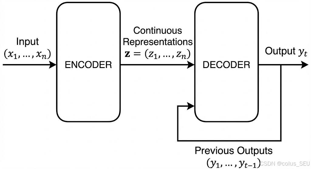
Most competitive neural sequence transduction models have an encoder-decoder structure. Here, the encoder maps an input sequence of symbol representations $(x_1, ..., x_n)$ to a sequence of continuous representations $\mathbf{z} = (z_1, ..., z_n)$ . Given $\mathbf{z}$ , the decoder then generates an output sequence $(y_1, ..., y_m)$ of symbols one element at a time. At each step the model is auto-regressive, consuming the previously generated symbols as additional input when generating the next.

auto-regressive，自回归，即利用一个变量过去的历史值，来预测它当前或未来的值。

Transformer 一样使用了编码解码架构。

3.1 Encoder and Decoder Stacks

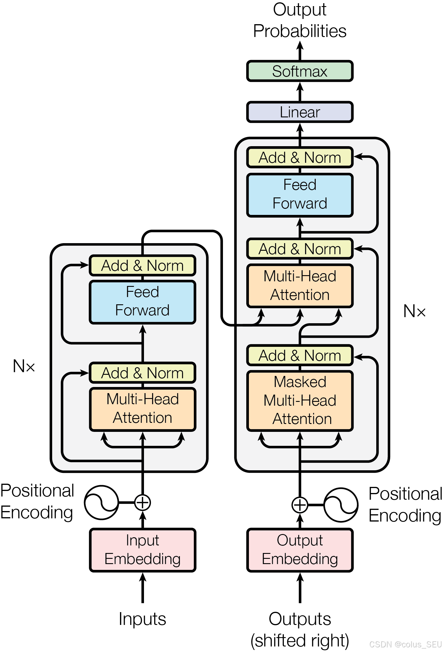
Encoder: The encoder is composed of a stack of N = 6 identical layers. Each layer has two sub-layers. The first is a multi-head self-attention mechanism, and the second is a simple, position-wise fully connected feed-forward network. We employ a residual connection around each of the two sub-layers, followed by layer normalization. That is, the output of each sub-layer is $\text{LayerNorm}(x + \text{Sublayer}(x))$ where $\text{Sublayer}(x)$ is the function implemented by the sub-layer itself. To facilitate these residual connections, all sub-layers in the model, as well as the embedding layers, produce outputs of dimension $d_{\text{model}} = 512$ .

Decoder: The decoder is also composed of a stack of N = 6 identical layers. In addition to the two sub-layers in each encoder layer, the decoder inserts a third sub-layer, which performs multi-head attention over the output of the encoder stack. Similar to the encoder, we employ residual connections around each of the sub-layers, followed by layer normalization. We also modify the self-attention sub-layer in the decoder stack to prevent positions from attending to subsequent positions. This masking, combined with fact that the output embeddings are offset by one position, ensures that the predictions for position i can depend only on the known outputs at positions less than i.

这里 Decoder 的 mask（掩码）的作用是：在训练时，我们一次性把正确答案（Ground Truth）输入给 Decoder。但是，在预测第 i 个词时，模型绝对不能“偷看”到 i 之后的内容。因此，作者引入了 Masking，把 i 之后的位置全部遮住（设为负无穷大），确保位置 i 只能关注到 <i 的位置。即 "auto-regressive"（自回归） 属性。

3.2 Attention

3.2.1 Scaled Dot product Attention 缩放点积注意力

公式介绍：

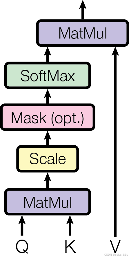
The input consists of queries and keys of dimension $d_k$ , and values of dimension $d_v$ . We compute the dot products of the query with all keys, divide each by $\sqrt{d_k}$ , and apply a softmax function to obtain the weights on the values.

In practice, we compute the attention function on a set of queries simultaneously, packed together into a matrix Q. The keys and values are also packed together into matrices K and V. We compute the matrix of outputs as:

$\text{Attention}(Q, K, V) = \text{softmax}\left(\frac{QK^T}{\sqrt{d_k}}\right)V$

要理解这个公式，首先需要知道三个矩阵的具体含义：Q (query), K (key), V (value)

Q：模型当前正在处理的 token，它拿着自己的特征去寻找“谁跟我有关系？”。

K：模型序列中所有 token 用来“被查询”的特征标志。

V：模型中token 真正包含的语义信息。如果它被选中了，它就把这些信息贡献出来。

该公式的核心逻辑是：拿着 Q 去和所有的 K 进行匹配（计算相似度），根据匹配程度（权重），把对应的 V 加权混合起来，就得到了最终的输出。

具体过程包括：

Step 1: 线性变换

Q, K, V 不是凭空产生的，它们都是由输入向量 X（或者是上一层的输出）通过三个不同的可学习权重矩阵投影得到的，且由于乘了不同的矩阵，它们所在的特征空间是不同的。

$Q = X W^Q$

$K = X W^K$

$V = X W^V$

Step 2: 计算相似度 (Dot Product QK^T)

将 Q 和 K 进行点积运算，得到一个分数矩阵（Score Matrix），表示“当前词” Q 关注“其他词” K 的程度。

Step 3: 缩放 (Scaling $\frac{1}{\sqrt{d_k}}$ )

Step 4: Softmax 之后乘 V

Softmax 将分数转化为概率分布（权重和为 1），这决定了模型在看每个词时的“注意力分配”。

然后用算出来的权重去乘 V：

如果 Q 和某个 K 极度相似，Softmax 接近 1，输出就几乎保留了该 K 对应的 V。

如果 Q 和某个 K 不相关，Softmax 接近 0，该 V 的信息就被过滤掉了。

为什么要缩放？

The two most commonly used attention functions are additive attention and dot-product (multiplicative) attention. Dot-product attention is identical to our algorithm, except for the scaling factor of $\frac{1}{\sqrt{d_k}}$ . Additive attention computes the compatibility function using a feed-forward network with a single hidden layer. While the two are similar in theoretical complexity, dot-product attention is much faster and more space-efficient in practice, since it can be implemented using highly optimized matrix multiplication code.

While for small values of $d_k$ the two mechanisms perform similarly, additive attention outperforms dot product attention without scaling for larger values of $d_k$ . We suspect that for large values of $d_k$ , the dot products grow large in magnitude, pushing the softmax function into regions where it has extremely small gradients. To counteract this effect, we scale the dot products by $\frac{1}{\sqrt{d_k}}$ .

首先我们要知道，常用的注意力机制有加性注意力和点积注意力，而缩放点积注意力，顾名思义，就是在点积注意力的基础上增加了缩放这个步骤。

加性注意力使用一个包含单隐藏层的前馈神经网络来计算 Q 和 K 之间的兼容性函数，它认为 Query 和 Key 是两个不同的向量，要计算它们的相似度，最好的办法是把它们拼在一起，扔进一个神经网络里算一算：

$$
\text{Score}(q, k) = v^T \tanh(W_1 q + W_2 k)
$$

或者简单理解为：MLP([q, k])

特点：

运算：涉及向量拼接、矩阵乘法、tanh 激活函数。

优点：即使维度很高也非常稳定（因为它有激活函数 tanh 限制数值范围）。

缺点：慢！它的计算难以高度并行化，因为它是专门的一个小神经网络。

而点积注意力认为向量的点积本身就代表了相似度：

$$
\text{Score}(q, k) = q^T k
$$

特点：

运算：纯粹的矩阵乘法 (Matrix Multiplication)。

优点：GPU 擅长矩阵乘法。这也是 Transformer 能够训练这么快、层数这么深的核心原因。

缺点：当维度 $d_k$ 很大时，点积结果会非常大（量级爆炸），导致 Softmax 的梯度消失。

为了解决点积结果的梯度消失问题，才使用了缩放机制。

如果还没有完全理解，可以继续看以下具体的例子：

假设有输入句子：I Love AI
- Token 1: "I"
- Token 2: "Love"
- Token 3: "AI"
假设维度 ( $d_{\text{model}}$ ): 4
假设 Query/Key/Value 维度 ( $d_q=d_k, d_v$ ): 也是 4

首先，我们将这 3 个词转换成向量，假设为：

$$
X = \begin{bmatrix} 1 & 0 & 1 & 0 \\ 0 & 1 & 0 & 1 \\ 1 & 1 & 0 & 0 \end{bmatrix} \begin{matrix} \leftarrow \text{"I"} \\ \leftarrow \text{"Love"} \\ \leftarrow \text{"AI"} \end{matrix}
$$

我们用三个不同的权重矩阵 ( $W^Q, W^K, W^V$ ) 对 X 进行变换，得到 Q, K, V，假设结果为：

Q (Query - "我想查什么"):

$$
Q = \begin{bmatrix} 2 & 0 & 1 & -1 \\ -1 & 2 & 0 & 1 \\ 0 & -1 & 2 & 0 \end{bmatrix} \begin{matrix} \leftarrow Q_{\text{"I"}} \\ \leftarrow Q_{\text{"Love"}} \\ \leftarrow Q_{\text{"AI"}} \end{matrix}
$$

K (Key - "我有什么标签"):

$$
K = \begin{bmatrix} -1 & 0 & 2 & 1 \\ 1 & -1 & 0 & 2 \\ 2 & 1 & -1 & 0 \end{bmatrix} \begin{matrix} \leftarrow K_{\text{"I"}} \\ \leftarrow K_{\text{"Love"}} \\ \leftarrow K_{\text{"AI"}} \end{matrix}
$$

V (Value - "我的内容是什么"):

$$
V = \begin{bmatrix} 2 & 1 & 0 & 1 \\ 1 & 2 & 1 & 0 \\ 3 & 1 & 2 & 1 \end{bmatrix} \begin{matrix} \leftarrow V_{\text{"I"}} \\ \leftarrow V_{\text{"Love"}} \\ \leftarrow V_{\text{"AI"}} \end{matrix}
$$

然后计算 Q 和 K 的点积，看看每个词对其他词的"关注度"。

$$
\text{Scores} = Q \cdot K^T = \begin{bmatrix} \mathbf{-1} & 0 & \mathbf{3} \\ \mathbf{2} & -1 & 0 \\ \mathbf{4} & 1 & -3 \end{bmatrix}
$$

解读第一行 (Token "I" 的视角):

"I" 对 "I" 的分数： $2\times(-1) + 0\times0 + 1\times2 + (-1)\times1 = \mathbf{-1}$
"I" 对 "Love" 的分数： $2\times1 + 0\times(-1) + 1\times0 + (-1)\times2 = \mathbf{0}$
"I" 对 "AI" 的分数： $2\times2 + 0\times1 + 1\times(-1) + (-1)\times0 = \mathbf{3}$ (最高分！说明 "I" 这个词在这个语境下最关注 "AI")

然后进行缩放 (Scaling)，即除以 $\sqrt{d_k} = \sqrt{4} = \mathbf{2}$ 。防止数值过大导致梯度消失。

$$
\text{Scaled Scores} = \begin{bmatrix} -0.5 & 0.0 & \mathbf{1.5} \\ \mathbf{1.0} & -0.5 & 0.0 \\ \mathbf{2.0} & 0.5 & -1.5 \end{bmatrix}
$$

对每一行进行 Softmax，转化为概率分布（和为 1）。这就是最终的 Attention Map。

$$
\text{Attention Weights} = \begin{bmatrix} 0.10 & 0.16 & \mathbf{0.74} \\ \mathbf{0.63} & 0.14 & 0.23 \\ \mathbf{0.80} & 0.18 & 0.02 \end{bmatrix} \begin{matrix} \leftarrow \text{"I" 把 74\% 的注意力给了 "AI"} \\ \leftarrow \text{"Love" 主要关注 "I" (63\%)} \\ \leftarrow \text{"AI" 主要关注 "I" (80\%)} \end{matrix}
$$

最后，用计算出的权重去乘 V 矩阵，得到最终输出 Z。以第一个词 "I" 的输出 $z_1$ 为例：

$$
z_1 = 0.10 \times V_{\text{"I"}} + 0.16 \times V_{\text{"Love"}} + 0.74 \times V_{\text{"AI"}} \\ = 0.10 \times [2, 1, 0, 1] + 0.16 \times [1, 2, 1, 0] + 0.74 \times [3, 1, 2, 1] \\ = [0.20, 0.10, 0.00, 0.10] + [0.16, 0.32, 0.16, 0.00] + [2.22, 0.74, 1.48, 0.74] \\ = [\mathbf{2.58}, \mathbf{1.16}, \mathbf{1.64}, \mathbf{0.84}]
$$

可以看到，"I" 的最终表示向量 [2.58, 1.16, 1.64, 0.84] 混合了三个词的信息。

3.2.2 Multi-head Attention 多头注意力

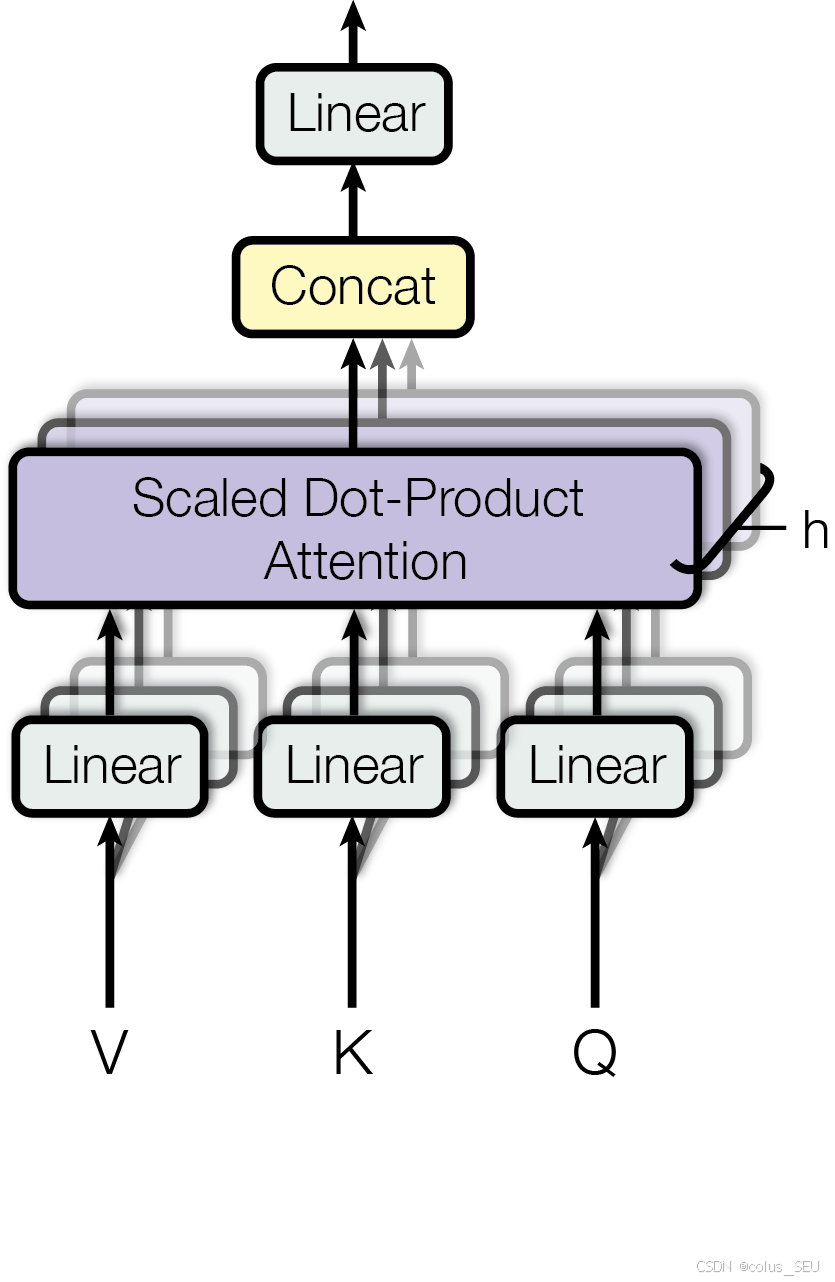
Instead of performing a single attention function with $d_{\text{model}}$ -dimensional keys, values and queries we found it beneficial to linearly project the queries, keys and values h times with different, learned linear projections to $d_k$ , $d_k$ and $d_v$ dimensions, respectively. On each of these projected versions of queries, keys and values we then perform the attention function in parallel, yielding $d_v$ -dimensional output values. These are concatenated（拼接） and once again projected（投影）, resulting in the final values, as depicted in Figure 2.

Multi-head attention allows the model to jointly attend to information from different representation subspaces at different positions. With a single attention head, averaging inhibits this.

$$
\text{MultiHead}(Q, K, V) = \text{Concat}(\text{head}_1, \ldots, \text{head}_h)W^O \\ \text{where head}_i = \text{Attention}(QW_i^Q, KW_i^K, VW_i^V)
$$

Where the projections are parameter matrices $W_i^Q \in \mathbb{R}^{d_{\text{model}} \times d_k}$ , $W_i^K \in \mathbb{R}^{d_{\text{model}} \times d_k}$ , $W_i^V \in \mathbb{R}^{d_{\text{model}} \times d_v}$ and $W^O \in \mathbb{R}^{hd_v \times d_{\text{model}}}$ .

In this work we employ h = 8 parallel attention layers, or heads. For each of these we use $d_k = d_v = d_{\text{model}}/h = 64$ . Due to the reduced dimension of each head, the total computational cost is similar to that of single-head attention with full dimensionality.

作者认为与其使用 $d_{\text{model}}$ 维度的 Key、Value 和 Query 执行单个注意力函数，不如将 Query、Key 和 Value 分别使用不同的、学习到的线性投影矩阵进行 h 次线性投影，分别映射到 $d_k$ 、 $d_k$ 和 $d_v$ 维度，这样做更有益处。

多头注意力机制允许模型联合关注来自不同位置的不同表征子空间的信息，而单头注意力机制由于平均化抑制了该能力。这里的不同表征子空间指的是通过 $W_i^Q, W_i^K, W_i^V$ 投影将数据映射到了不同的子空间。

该论文采用 h=8 个并行的注意力层（即“头”）。对每一个头，用 $d_k = d_v = d_{\text{model}}/h = 64$ 。由于每个头的维度减小了，总的计算成本与具有全维度的单头注意力相似。即单头的话，进行一次注意力计算，向量长度为 512；而多头进行8比注意力计算，但每次向量长度只有原来的 $\frac{1}{8}$ ，所以总的计算成本不变，但表达能力却增强了。

我们继续用 “I love AI” 这个例子，序列：["I", "Love", "AI"]，维度 $d_{\text{model}}=4$

$$
X = \begin{bmatrix} 1 & 0 & 1 & 0 \\ 0 & 1 & 0 & 1 \\ 1 & 1 & 0 & 0 \end{bmatrix} \begin{matrix} \leftarrow \text{"I"} \\ \leftarrow \text{"Love"} \\ \leftarrow \text{"AI"} \end{matrix}
$$

对单头注意力，之前算的就是单头注意力的结果，（以 $z_1$ 为例） $z_{\text{single}} = [\mathbf{2.58}, \mathbf{1.16}, \mathbf{1.64}, \mathbf{0.84}]$

对多头注意力，假设我们有两个头

设定：Head 1 专注于输入的前两个维度。 Head 2 专注于输入的后两个维度。分别计算如下：

1. 投影权重 ( $W_1$ )

这是 Head 1 的“眼镜”，用来提取特征。

$$
W_1^Q = \begin{bmatrix} 1 & 0 \\ 0 & 1 \\ 0 & 0 \\ 0 & 0 \end{bmatrix}, \quad W_1^K = \begin{bmatrix} 1 & 0 \\ 0 & 1 \\ 1 & 0 \\ 0 & 0 \end{bmatrix}, \quad W_1^V = \begin{bmatrix} 1 & 1 \\ 0 & 1 \\ 0 & 0 \\ 1 & 0 \end{bmatrix}
$$

2. 投影结果 ( $Q_1, K_1, V_1$ )

通过 $X \cdot W_1$ 计算得到：

$$
Q_1 = \begin{bmatrix} 1 & 0 \\ 0 & 1 \\ 1 & 1 \end{bmatrix}, \quad K_1 = \begin{bmatrix} 2 & 0 \\ 0 & 1 \\ 1 & 1 \end{bmatrix}, \quad V_1 = \begin{bmatrix} 1 & 1 \\ 1 & 1 \\ 1 & 2 \end{bmatrix}
$$

3. 注意力分数与权重

原始分数 ( $Q_1 K_1^T$ )：

$$
\text{Scores}_1 = \begin{bmatrix} 2 & 0 & 1 \\ 0 & 1 & 1 \\ 2 & 1 & 2 \end{bmatrix}
$$
缩放后分数 ( $\text{Scores}_1 / \sqrt{2}$ )：

$$
\text{Scaled}_1 = \begin{bmatrix} 1.41 & 0.00 & 0.71 \\ 0.00 & 0.71 & 0.71 \\ 1.41 & 0.71 & 1.41 \end{bmatrix}
$$
归一化权重 (Softmax, $\text{Attn}_1$ )： Head 1 最终的注意力分布矩阵

$$
\text{Attn}_1 = \begin{bmatrix} \mathbf{0.58} & 0.14 & 0.28 \\ 0.20 & \mathbf{0.40} & \mathbf{0.40} \\ \mathbf{0.40} & 0.20 & \mathbf{0.40} \end{bmatrix} \begin{matrix} \leftarrow \text{"I" 主要关注自己} \\ \leftarrow \text{"Love" 均分关注Love和AI} \\ \leftarrow \text{"AI" 均分关注I和AI} \end{matrix}
$$

4. Head 1 输出 ( $Z_1 = \text{Attn}_1 \cdot V_1$ )

$$
Z_1 = \begin{bmatrix} 1.00 & 1.28 \\ 1.00 & 1.40 \\ 1.00 & 1.40 \end{bmatrix}
$$

1. 投影权重 ( $W_2$ )

这是 Head 2 的“眼镜”。

$$
W_2^Q = \begin{bmatrix} 0 & 0 \\ 0 & 0 \\ 1 & 0 \\ 0 & 1 \end{bmatrix}, \quad W_2^K = \begin{bmatrix} 0 & 0 \\ 0 & 0 \\ 0 & 1 \\ 1 & 0 \end{bmatrix}, \quad W_2^V = \begin{bmatrix} 1 & 0 \\ 1 & 0 \\ 0 & 1 \\ 0 & 1 \end{bmatrix}
$$

2. 投影结果 ( $Q_2, K_2, V_2$ )

$$
Q_2 = \begin{bmatrix} 1 & 0 \\ 0 & 1 \\ 0 & 0 \end{bmatrix}, \quad K_2 = \begin{bmatrix} 0 & 1 \\ 1 & 0 \\ 0 & 0 \end{bmatrix}, \quad V_2 = \begin{bmatrix} 1 & 1 \\ 1 & 1 \\ 2 & 0 \end{bmatrix}
$$

3. 注意力分数与权重

原始分数 ( $Q_2 K_2^T$ )：

$$
\text{Scores}_2 = \begin{bmatrix} 0 & 1 & 0 \\ 1 & 0 & 0 \\ 0 & 0 & 0 \end{bmatrix}
$$
缩放后分数 ( $\text{Scores}_2 / \sqrt{2}$ )：

$$
\text{Scaled}_2 = \begin{bmatrix} 0.00 & 0.71 & 0.00 \\ 0.71 & 0.00 & 0.00 \\ 0.00 & 0.00 & 0.00 \end{bmatrix}
$$
归一化权重 (Softmax, $\text{Attn}_2$ )：

$$
\text{Attn}_2 = \begin{bmatrix} 0.25 & \mathbf{0.50} & 0.25 \\ \mathbf{0.50} & 0.25 & 0.25 \\ 0.33 & 0.33 & 0.33 \end{bmatrix} \begin{matrix} \leftarrow \text{"I" 强烈关注 "Love"} \\ \leftarrow \text{"Love" 强烈关注 "I"} \\ \leftarrow \text{"AI" 平均关注} \end{matrix}
$$

4. Head 2 输出 ( $Z_2 = \text{Attn}_2 \cdot V_2$ )

$$
Z_2 = \begin{bmatrix} 1.25 & 0.75 \\ 1.25 & 0.75 \\ 1.33 & 0.67 \end{bmatrix}
$$

最终融合 (Final Output)

将 $Z_1 (3\times2)$ 和 $Z_2 (3\times2)$ 横向拼在一起，得到 3x4 的矩阵：

$$
Z_{\text{concat}} = \begin{bmatrix} \mathbf{1.00} & \mathbf{1.28} & \mathbf{1.25} & \mathbf{0.75} \\ 1.00 & 1.40 & 1.25 & 0.75 \\ 1.00 & 1.40 & 1.33 & 0.67 \end{bmatrix} \begin{matrix} \leftarrow Z_{\text{final}} \text{ (I)} \\ \leftarrow Z_{\text{final}} \text{ (Love)} \\ \leftarrow Z_{\text{final}} \text{ (AI)} \end{matrix}
$$

(注：此处省略了 $W^O$ 的乘法，假设 $W^O$ 为单位矩阵，所以 $Z_{\text{final}} = Z_{\text{concat}}$ )

3.2.3 Applications of Attention in our Model

从架构图中可以发现，多头注意力一共用在了三个地方。（架构图中橙黄色的部分）

The Transformer uses multi-head attention in three different ways:

In "encoder-decoder attention" layers, the queries come from the previous decoder layer, and the memory keys and values come from the output of the encoder. This allows every position in the decoder to attend over all positions in the input sequence. This mimics the typical encoder-decoder attention mechanisms in sequence-to-sequence models.
The encoder contains self-attention layers. In a self-attention layer all of the keys, values and queries come from the same place, in this case, the output of the previous layer in the encoder. Each position in the encoder can attend to all positions in the previous layer of the encoder.
Similarly, self-attention layers in the decoder allow each position in the decoder to attend to all positions in the decoder up to and including that position. We need to prevent leftward information flow in the decoder to preserve the auto-regressive property. We implement this inside of scaled dot-product attention by masking out (setting to $-\infty$ ) all values in the input of the softmax which correspond to illegal connections.

注意力类型所在模块 Q来源 K/V来源掩码作用范围

Encoder-Decoder Attention 解码器右侧上层前一解码层编码器输出无全源序列

Encoder Self-Attention 编码器左侧前一编码层前一编码层无全序列双向

Masked Decoder Self-Attention 解码器右侧下层前一解码层前一解码层有（上三角掩码）当前位置左侧

注意力类型	所在模块	Q来源	K/V来源	掩码	作用范围
Encoder-Decoder Attention	解码器右侧上层	前一解码层	编码器输出	无	全源序列
Encoder Self-Attention	编码器左侧	前一编码层	前一编码层	无	全序列双向
Masked Decoder Self-Attention	解码器右侧下层	前一解码层	前一解码层	有（上三角掩码）	当前位置左侧

3.3 Position-wise Feed-Forward Networks

基于位置的前馈神经网络（架构图中蓝色的部分）

In addition to attention sub-layers, each of the layers in our encoder and decoder contains a fully connected feed-forward network, which is applied to each position separately and identically. This consists of two linear transformations with a ReLU activation in between.

$$
\text{FFN}(x) = \max(0, xW_1 + b_1)W_2 + b_2
$$

这个结构可以拆解为三步：

第一层线性变换 (Linear Expansion): 输入 x 乘以矩阵 $W_1$ 并加上偏置 $b_1$ 。这一步通常会将维度放大。

非线性激活 (ReLU): 使用 ReLU 函数 ( $\max(0, z)$ ) 进行激活。这是 Transformer 每一层中引入非线性的关键来源（Attention 本质上是线性加权）。

第二层线性变换 (Linear Projection): 乘以矩阵 $W_2$ 并加上偏置 $b_2$ ，将维度还原回输入的大小。

While the linear transformations are the same across different positions, they use different parameters from layer to layer. Another way of describing this is as two convolutions with kernel size 1. The dimensionality of input and output is $d_{\text{model}} = 512$ , and the inner-layer has dimensionality $d_{ff} = 2048$ .

直观理解：这个网络是一个“宽体”结构。数据流进来是 512 维，中间突然膨胀到 2048 维，经过复杂的非线性变换后，再压缩回 512 维。

这种 窄 \to 宽 \to 窄 的结构（类似倒置的瓶颈层）允许模型在更高维的空间里组合特征，增加模型的拟合能力。

这里有两个中重要的问题：

一、什么是 "Position-wise" (基于位置)？

文中提到："applied to each position separately and identically."

Separately (独立地):
- Attention 负责处理词与词之间的关系（"I" 看到了 "AI"）。
- FFN 则是只关注当前词自己。它把每个词的向量单独拿出来，扔进这个 MLP 里算一遍，完全不管旁边的词是谁。例如，处理 "I" 时，FFN 不知道 "Love" 的存在。
Identically (相同地):
- 虽然每个词是独立算的，但它们共用同一套参数 ( $W_1, b_1, W_2, b_2$ )。即无论你在句子的第 1 个位置还是第 100 个位置，处理你的“加工厂”是完全一样的。

文中提到这也可以被描述为 "two convolutions with kernel size 1"（两个核大小为 1 的卷积）。这就是在说：我们在序列长度方向上扫描，但只看当前点（Kernel size=1），对特征通道（Channel）做全连接变换。

二、既然 Attention 已经聚合了上下文信息，为什么还要接一个 FFN？

Attention 的局限： Attention 只是在做“加权平均”。它把其他词的特征搬运过来，混合在一起。这本质上还是在特征空间里做线性组合。
FFN 的作用： FFN 引入了非线性（ReLU）和特征变换能力，消化 Attention 搬运过来的信息。
- Attention: "嘿，我发现 'bank' 这个词在这里应该和 'river' 关联，我把 'river' 的特征加进来了。"
- FFN: "收到。结合 'river' 的特征，我现在要把 'bank' 的语义从'银行'转换成'河岸'，并存入新的维度中。"

3.4 Embeddings and Softmax

（架构图中两个红色的embedding层和一个绿色的softmax层）

Similarly to other sequence transduction models, we use learned embeddings to convert the input tokens and output tokens to vectors of dimension $d_{\text{model}}$ . We also use the usual learned linear transformation and softmax function to convert the decoder output to predicted next-token probabilities. In our model, we share the same weight matrix between the two embedding layers and the pre-softmax linear transformation. In the embedding layers, we multiply those weights by $\sqrt{d_{\text{model}}}$ .

和其他序列模型一样，Transformer 的 Embedding 层一样负责将离散的 Token（如单词 "AI" ）转换为 $d_{model}$ 维的向量。

完成线性变换后，模型用 softmax 函数将 decoder 的输出转换为下一个 token 的预测概率分布。

两个嵌入层（Encoder 输入 Embedding 和 Decoder 输入 Embedding）以及 Pre-softmax 线性变换层，这三个层共享同一个权重矩阵。理由：输入的词向量空间和输出的词向量空间理论上应该是同构的，例如，“Cat”作为输入时的语义向量和预测输出时的“Cat”向量是一致的，换句话说，相同的 token ，嵌入向量必然相同。并且这样做可以使参数量大幅减少。

在 Embedding 层中，将权重乘以 $\sqrt{d_{model}}$ 。这样做是因为初始化时，Embedding 权重的方差通常比较小（为了保持初始数值稳定）。但在 Transformer 内部，尤其是加上了 Positional Encoding 之后，数值的量级需要匹配。Positional Encoding 的数值范围大约在 [-1, 1] 之间。如果 Embedding 的数值太小（接近 0），加上位置编码后，语义信息就会被位置信息淹没。乘以 $\sqrt{d_{model}}$ （比如 $\sqrt{512} \approx 22.6$ ）可以将 Embedding 的数值放大，使其与 Positional Encoding 的数值量级相当，从而平衡“语义信息”和“位置信息”的权重。

3.5 Positional Encoding

加在 Embedding 层之后。

Since our model contains no recurrence and no convolution, in order for the model to make use of the order of the sequence, we must inject some information about the relative or absolute position of the tokens in the sequence. To this end, we add "positional encodings" to the input embeddings at the bottoms of the encoder and decoder stacks. The positional encodings have the same dimension $d_{\text{model}}$ as the embeddings, so that the two can be summed. There are many choices of positional encodings, learned and fixed.

在 RNN 中，模型按顺序逐个处理词语，该方式天然地包含了顺序信息。但是 Transformer 摒弃了循环和卷积结构，因此必须想办法引入序列中 token 的顺序信息。

Transformer 通过在 input Embedding 之后直接加一个相同维度（ $d_{\text{model}}$ ）位置编码向量来引入 token 在序列中绝对或相对位置的信息。

In this work, we use sine and cosine functions of different frequencies:

$$
PE_{(pos,2i)} = sin(pos/10000^{2i/d_{\text{model}}}) \\ PE_{(pos,2i+1)} = cos(pos/10000^{2i/d_{\text{model}}})
$$

where pos is the position and i is the dimension. That is, each dimension of the positional encoding corresponds to a sinusoid. The wavelengths form a geometric progression from $2\pi$ to $10000 \cdot 2\pi$ . We chose this function because we hypothesized it would allow the model to easily learn to attend by relative positions, since for any fixed offset k, $PE_{pos+k}$ can be represented as a linear function of $PE_{pos}$ .

论文并没有使用简单的整数（如 1, 2, 3...）来标记位置，而是设计了一组基于正弦（Sine）和余弦（Cosine）函数的频率系统，并给出了对于位置 pos 和维度 i，位置编码 PE 的计算公式：

pos：词在句子中的位置（例如第 1 个词，第 2 个词）。

i：向量维度的索引（例如 $d_{model}=512$ ，则 i 范围是 0 到 255）。

2i 和 2i+1：分别代表偶数维度和奇数维度。

直观理解：这就好比每一个维度都是一个按照不同频率旋转的时钟指针。

波长形成了一个从 $2\pi$ 到 $10000 \cdot 2\pi$ 的几何级数。

在低维度（i 较小），波长短，数值变化频率高。

在高维度（i 较大），波长长，数值变化频率低。

作者在文中给出了选择这种特定函数的两个主要理由：

A. 易于学习相对位置 (Relative Position)

作者假设这种函数形式可以让模型更容易地学习到相对位置的注意力模式。数学上，对于任何固定的偏移量 k，位置 pos+k 的编码向量 $PE_{pos+k}$ 可以表示为位置 pos 的编码向量 $PE_{pos}$ 的线性函数（Linear Function）。这意味着模型只需要学习一个线性变换矩阵，就能捕捉到“Token A 在 Token B 后面 k 个位置”这样的关系。该线性变换矩阵的推导如下：

为了方便推导，我们设定角频率 $\omega_i = \frac{1}{10000^{2i/d_{model}}}$

那么对于维度 2i 和 2i+1，位置编码向量 $PE_{pos}$ 的分量可以写为：

$$
\begin{align} PE_{(pos, 2i)} &= \sin(\omega_i \cdot pos) \\ PE_{(pos, 2i+1)} &= \cos(\omega_i \cdot pos) \end{align}
$$

我们需要证明：对于位置 pos+k，其编码向量 $PE_{pos+k}$ 可以通过一个与 pos 无关（只与 k 有关）的矩阵 $M_k$ 乘以 $PE_{pos}$ 得到：

$$
PE_{pos+k} = M_k \cdot PE_{pos}
$$

考察位置 pos+k 处的编码：

$$
\begin{align} PE_{(pos+k, 2i)} &= \sin(\omega_i (pos + k)) \\ PE_{(pos+k, 2i+1)} &= \cos(\omega_i (pos + k)) \end{align}
$$

对于正弦分量（偶数维度）：

$$
\begin{aligned} PE_{(pos+k, 2i)} &= \sin(\omega_i pos + \omega_i k) \\ &= \sin(\omega_i pos)\cos(\omega_i k) + \cos(\omega_i pos)\sin(\omega_i k) \\ &= PE_{(pos, 2i)} \cdot \cos(\omega_i k) + PE_{(pos, 2i+1)} \cdot \sin(\omega_i k) \end{aligned}
$$

对于余弦分量（奇数维度）：

$$
\begin{aligned} PE_{(pos+k, 2i+1)} &= \cos(\omega_i pos + \omega_i k) \\ &= \cos(\omega_i pos)\cos(\omega_i k) - \sin(\omega_i pos)\sin(\omega_i k) \\ &= PE_{(pos, 2i+1)} \cdot \cos(\omega_i k) - PE_{(pos, 2i)} \cdot \sin(\omega_i k) \end{aligned}
$$

将上述两个等式写成矩阵乘法的形式。对于第 i 组频率，我们有：

$$
\begin{bmatrix} PE_{(pos+k, 2i)} \\ PE_{(pos+k, 2i+1)} \end{bmatrix} = \begin{bmatrix} \cos(\omega_i k) & \sin(\omega_i k) \\ -\sin(\omega_i k) & \cos(\omega_i k) \end{bmatrix} \cdot \begin{bmatrix} PE_{(pos, 2i)} \\ PE_{(pos, 2i+1)} \end{bmatrix}
$$

上面的矩阵 \begin{bmatrix} \cos(\omega_i k) & \sin(\omega_i k) \\ -\sin(\omega_i k) & \cos(\omega_i k) \end{bmatrix} 就是论文中隐含提到的线性变换矩阵。这是一个标准的旋转矩阵。这个旋转矩阵中的元素只包含 $\omega_i$ （固定的频率）和 $k$ （相对偏移量）。它完全不包含 pos。这意味着，Transformer 的注意力机制（通常包含线性变换 $W^Q$ , $W^K$ ）可以很容易地学习到这个旋转矩阵。只要模型学到了这个旋转操作，它就能在任何绝对位置 pos 上，轻松地“关注”到距离它 k 个单位的那个词，而不需要针对每个 pos 单独学习规则。

B. 长度外推能力 (Extrapolation)

作者选择正弦版本也是因为它允许模型处理比训练期间遇到的序列更长的序列。如果使用训练好的“学习型位置嵌入”（Learned Embeddings），当推理时遇到比训练集最长句子还长的序列时，模型可能无法处理那些未见过的位置索引。而正弦函数是周期性且连续的，理论上可以延伸。

We also experimented with using learned positional embeddings instead, and found that the two versions produced nearly identical results (see Table 3 row (E)). We chose the sinusoidal version because it may allow the model to extrapolate to sequence lengths longer than the ones encountered during training.

作者还尝试了另一种常见的方法：可学习的位置嵌入 (Learned Positional Embeddings) 。

这种方法就像学习词向量一样，让神经网络自己去学习每个位置应该对应的向量。实验结果显示，正弦编码与可学习嵌入效果相似。但作者最终选择了正弦/余弦编码，正是因为上述提到的“长度外推能力” 。

4. Why Self-Attention

In this section we compare various aspects of self-attention layers to the recurrent and convolutional layers commonly used for mapping one variable-length sequence of symbol representations $(x_1, ..., x_n)$ to another sequence of equal length $(z_1, ..., z_n)$ , with $x_i, z_i \in \mathbb{R}^d$ , such as a hidden layer in a typical sequence transduction encoder or decoder. Motivating our use of self-attention we consider three desiderata.

One is the total computational complexity per layer. Another is the amount of computation that can be parallelized, as measured by the minimum number of sequential operations required.

The third is the path length between long-range dependencies in the network. Learning long-range dependencies is a key challenge in many sequence transduction tasks. One key factor affecting the ability to learn such dependencies is the length of the paths forward and backward signals have to traverse in the network. The shorter these paths between any combination of positions in the input and output sequences, the easier it is to learn long-range dependencies. Hence we also compare the maximum path length between any two input and output positions in networks composed of the different layer types.

作者在比较用于将变长输入序列 $(x_1, ..., x_n)$ 映射到等长输出序列 $(z_1, ..., z_n)$ 的，通常存在于用于序列转导的编码解码结构中的自注意力层，循环层，卷积层时，使用了三个指标：

每一层的计算复杂度；

并行化能力；

长距离依赖的路径长度：这是很多序列任务的关键挑战。网络中信号在两个位置之间传输必须经过的路径越短，模型就越容易学习到长距离的依赖关系。

As noted in Table 1, a self-attention layer connects all positions with a constant number of sequentially executed operations, whereas a recurrent layer requires O(n) sequential operations. In terms of computational complexity, self-attention layers are faster than recurrent layers when the sequence length n is smaller than the representation dimensionality d, which is most often the case with sentence representations used by state-of-the-art models in machine translations, such as word-piece and byte-pair representations. To improve computational performance for tasks involving very long sequences, self-attention could be restricted to considering only a neighborhood of size r in the input sequence centered around the respective output position. This would increase the maximum path length to $O(n/r)$ . We plan to investigate this approach further in future work.

A single convolutional layer with kernel width $k < n$ does not connect all pairs of input and output positions. Doing so requires a stack of O(n/k) convolutional layers in the case of contiguous kernels, or $O(\log_k(n))$ in the case of dilated convolutions, increasing the length of the longest paths between any two positions in the network. Convolutional layers are generally more expensive than recurrent layers, by a factor of k. Separable convolutions, however, decrease the complexity considerably, to $O(k \cdot n \cdot d + n \cdot d^2)$ . Even with $k = n$ , however, the complexity of a separable convolution is equal to the combination of a self-attention layer and a point-wise feed-forward layer, the approach we take in our model.

论文通过对比 Table 1 得出以下结论：

A. 路径长度 (Path Length)

自注意力机制 (Self-Attention)：胜出。它将所有位置连接起来的操作数是常数级 O(1) 。这意味着序列中任意两个词之间的距离都是一步直达，非常有利于学习长距离依赖。

循环网络 (RNN)：路径长度为 O(n) 。信号必须按时间步逐个传递，长距离依赖的学习更加困难。

卷积网络 (CNN)：通常需要堆叠多层才能覆盖整个序列。对于卷积核宽度为 k 的网络，路径长度通常是 $O(log_k(n))$ 或 $O(n/k)$ 。

B. 并行化操作 (Sequential Operations)

自注意力机制：胜出。顺序操作数为 O(1) 。整个序列的注意力计算可以并行完成。

循环网络：顺序操作数为 O(n) 。必须等待前一个时间步计算完成才能计算下一个，严重限制了并行训练的效率。

C. 计算复杂度 (Complexity per Layer)

自注意力机制：复杂度为 $O(n^2 \cdot d)$ 。

循环网络：复杂度为 $O(n \cdot d^2)$ 。

对比结论：当序列长度 n 小于表示维度 d 时（这是机器翻译模型中常见的情况，例如 word-piece 或 byte-pair 表示），自注意力层比循环层在计算上更快。

针对超长序列的优化：为了处理非常长的序列，作者提到可以将自注意力限制在以输出位置为中心的邻域 r 内（Restricted Self-Attention），但这会牺牲一部分最大路径长度优势。

D. 卷积层 (Convolutional Layers) 的劣势

单层卷积（核宽 k < n）无法连接所有输入和输出对。

需要堆叠 O(n/k) 层卷积层或使用空洞卷积才能覆盖全图，这增加了路径长度。

卷积层的计算代价通常比循环层高 k 倍。虽然可分离卷积（Separable Convolutions）可以降低复杂度，但即便在 k=n 的极端情况下，其复杂度也仅通过结合自注意力和前馈层的方式才能达到相当的水平。

As side benefit, self-attention could yield more interpretable models. We inspect attention distributions from our models and present and discuss examples in the appendix. Not only do individual attention heads clearly learn to perform different tasks, many appear to exhibit behavior related to the syntactic and semantic structure of the sentences.

除了上述性能指标，作者还指出自注意力模型具有更好的可解释性 ：通过检查注意力分布（Attention Distributions），可以直接观察模型在关注什么。

The Annotated Transformer

本文详细解读了 Transformer 的具体内容，如需聚焦其实现请参考：The Annotated Transformer

2048 AI社区

有“AI”的1024 = 2048，欢迎大家加入2048 AI社区

更多推荐

Prompt，除了使用外，你了解其核心原理么？

是的，除了日常“用”提示词之外，我对它的底层机制有比较系统的理解。Prompt Engineering 之所以在 2023–2026 年成为大模型时代最实用、最“玄学”又最科学的技能之一，是因为它本质上在操控 Transformer 架构的，而非修改模型权重。下面从最底层原理解释为什么“改几个词、加几句话”就能让模型表现天差地别（基于 Transformer 自注意力 + 预训练 + 后训练机制）