大模型FLOPs利用率_MFU计算方法与注意事项
MFU(Model Flop Utilization,模型浮点运算利用率)是衡量大模型训练 / 推理效率的核心指标,用于量化硬件(如 GPU)的浮点运算能力被模型实际利用的比例。其计算原理围绕 “理论最大算力” 与 “模型实际消耗算力” 的比值展开,直接反映了硬件资源的利用效率。在深度学习领域,评估模型的计算量通常涉及到多个指标,其中MACs(Multiply-Accumulate Operati
作者:昇腾实战派 x 3号小金鱼
摘要
MFU(Model Flop Utilization,模型浮点运算利用率)是衡量大模型训练 / 推理效率的核心指标,用于量化硬件(如 GPU)的浮点运算能力被模型实际利用的比例。其计算原理围绕 “理论最大算力” 与 “模型实际消耗算力” 的比值展开,直接反映了硬件资源的利用效率。在深度学习领域,评估模型的计算量通常涉及到多个指标,其中MACs(Multiply-Accumulate Operations)和FLOPs(Floating Point Operations)是两个核心概念。MACs:是Multiply ACcumulate operations的简称,又简称为MAdd,翻译为“累加乘积操作数”,一个MACs包含一个乘法操作和一个加法操作,因此1个MACs约等于2个FLOPs。
当一个新模型要计算MFU,如何快速计算模型的flops呢? 计算model_flops对很多人而言是一个繁琐的事情,为了提升MFU的计算效率,因此我们整理了常见模块的flops计算方法。本文一共2个章节,第一章节为针对常见不同模型组件Model Flops计算方法,第二章节为场景补充说明(参数冻结、重计算、变长序列等)。
该分析材料可能存在部分理解失准的地方,欢迎大家交流指正。
一、Model Flops计算方法
根据不同需求场景提供几种MFU计算方法如下图:
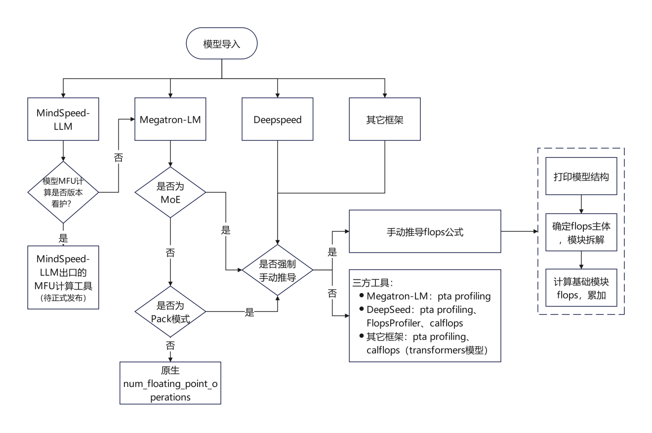
备注:手动推导flops公式可见1.1~1.2章节,三方工具见1.3章节和1.4章节,分别对应“常见三方工具”和“其它三方工具”。
1.1 传统小模型
1.1.1 Conv
常见的Conv类型包括conv1d、conv2d、conv3d等,通常具有不同的padding参数(例如:指定具体padding值、valid、same等);此外除了前述传统卷积以外,还有分组卷积、空洞卷积等,它们的计算逻辑存在差异,因此对应的model_flops计算逻辑也存在不同。
简单案例:为了说明卷积计算对model flops计算一般思路,以如下conv2d算子进行示例说明:
- 输入数据维度:
- 输入:[B, input_dim, W, H]
- 卷积核: [output_dim, input_dim,k_w, k_h]
- padding类型:same(paddding)
- 输出维度:根据上述输入维度容易计算输出维度为:[B, output_dim, W, H]
- 一般计算思路: torch.numel(output_tensor) × conv_per_position_macs,前者表示卷积操作输出张量中包含的元素总个数,后者表示获取每个元素对应的乘加计算次数。
- 计算结果:上述示例conv_per_position_macs=k_w×k_h×input_dim,MACs=(B×output_dim×W×H)×(k_w×k_h×input_dim)
计算代码:
输入参数说明:
- input:输入张量(shape:[N, C_in, D1, D2, …],N = 批次,C_in = 输入通道,D1/D2 = 空间维度);
- weight:卷积核张量(shape:[C_out, C_in/groups, K1, K2, …],C_out = 输出通道,K1/K2 = 卷积核空间尺
- bias:偏置张量(可选,shape:[C_out]);
- stride:步幅(int 或 tuple,如 Conv2d 中 (2,2));
- padding:填充(int/tuple/str,支持 ‘valid’/‘same’ 模式);
- dilation:空洞率(int 或 tuple,空洞卷积时 > 1);
- groups:分组卷积参数(默认 1,即普通卷积);
def _conv_flops_compute(input, weight, bias=None, stride=1, padding=0, dilation=1, groups=1):
    assert weight.shape[1] * groups == input.shape[1]
    batch_size = input.shape[0]  # 批次大小 N
    in_channels = input.shape[1]  # 输入通道数 C_in
    out_channels = weight.shape[0]  # 输出通道数 C_out
    kernel_dims = list(weight.shape[2:])  # 卷积核的空间维度(如 Conv2d 为 [K_h, K_w])
    input_dims = list(input.shape[2:])  # 输入张量的空间维度(如 Conv2d 为 [H_in, W_in])

    length = len(input_dims)  # 空间维度数量(1=Conv1d,2=Conv2d,3=Conv3d)

    # 1. 处理 stride:若为 int,扩展为对应维度的 tuple(如 Conv2d 中 stride=2 → (2,2))
    strides = stride if type(stride) is tuple else (stride, ) * length
    # 2. 处理 dilation:逻辑同 stride(如 dilation=1 → (1,1))
    dilations = dilation if type(dilation) is tuple else (dilation, ) * length

    # 3. 处理 padding:支持 'valid'/'same'/int/tuple 四种格式
    if isinstance(padding, str):
        if padding == 'valid':
            paddings = (0, ) * length  # valid 模式:无填充
        elif padding == 'same':
            paddings = ()
            # same 模式:计算每个维度的填充量(确保输出维度 = 输入维度 ÷ stride,向上取整)
            for d, k in zip(dilations, kernel_dims):
                total_padding = d * (k - 1)  # 空洞卷积下的有效卷积核覆盖范围
                paddings += (total_padding // 2, )  # 左右/上下各填充一半(整除处理)
    elif isinstance(padding, tuple):
        paddings = padding  # 直接使用 tuple 格式的填充(如 (1,1))
    else:
        paddings = (padding, ) * length  # int 格式扩展为 tuple(如 padding=1 → (1,1))

        output_dims = []
        for idx, input_dim in enumerate(input_dims):
            # 通用卷积输出维度公式(适配 1D/2D/3D + 空洞卷积 + 任意 padding/stride)
            output_dim = (input_dim + 2 * paddings[idx] - (dilations[idx] * (kernel_dims[idx] - 1) + 1)) // strides[idx] + 1
            output_dims.append(output_dim)

        filters_per_channel = out_channels // groups  # 每组的输出通道数(分组卷积核心)
        # 单个输出位置的 MACs:卷积核参数数(乘法次数=参数数,加法次数=参数数-1,工程上合并为 1 个 MAC/参数)
        conv_per_position_macs = int(_prod(kernel_dims)) * in_channels * filters_per_channel
        active_elements_count = batch_size * int(_prod(output_dims))  # 输出总元素数(N × 输出空间维度乘积)
        overall_conv_macs = conv_per_position_macs * active_elements_count  # 核心卷积的总 MACs

        overall_conv_flops = 2 * overall_conv_macs

        bias_flops = 0
        if bias is not None:
            bias_flops = out_channels * active_elements_count

    return int(overall_conv_flops + bias_flops), int(overall_conv_macs)
1.1.2 RNN
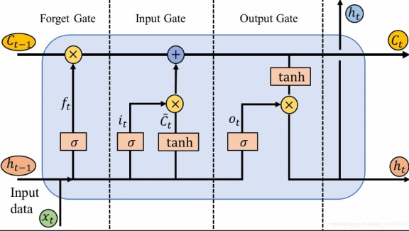
常见RNN结构包括:朴素RNN、LSTM、GRU等,系列变种结构中门控数量是典型特征之一,其中GRU有3个门控,LSTM有4个门控。
模型结构:
朴素RNN计算逻辑:
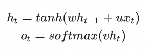
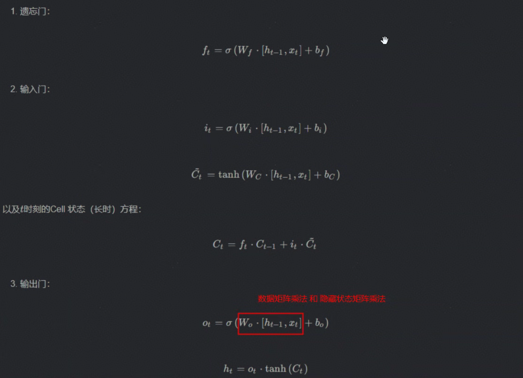
以LSTM为例模型结构和计算公式如下所示:
计算代码:
输入参数说明:
- input_size:输入特征维度(如文本序列的嵌入维度);
- hidden_size:隐藏层维度(RNN 核心参数,决定隐藏状态的维度);
- gates_size:门控数量 × hidden_size(如 LSTM 有 4 个门,gates_size=4×hidden_size;GRU 有 3 个门,gates_size=3×hidden_size);
- seq_length:序列长度(如文本序列的 token 数);
- batch_size:批次大小;
- num_layers:RNN 层数;
- bidirectional:是否双向(双向时 FLOPs 翻倍)。
示例代码说明:根据input维度和传入的rnn模型,逐层计算model_flops
def _rnn_forward_hook(rnn_module, input, output):
    flops = 0  # 初始化 FLOPs 计数器
    # input 是 tuple:包含待处理的序列(input[0])和可选的初始隐藏状态(input[1])
    inp = input[0]
    batch_size = inp.shape[0]  # 批次大小 N(输入张量 shape:[batch_size, seq_length, input_size])
    seq_length = inp.shape[1]  # 序列长度 L(输入序列的时间步数量)
    num_layers = rnn_module.num_layers  # RNN 层数(如 2 层 RNN)

    # 循环计算每一层的 FLOPs(RNN 是层叠结构,每层独立计算)
    for i in range(num_layers):
        # 获取当前层的输入权重矩阵 w_ih(shape:[gates_size, input_size])
        w_ih = rnn_module.__getattr__("weight_ih_l" + str(i))
        # 获取当前层的隐藏状态权重矩阵 w_hh(shape:[gates_size, hidden_size])
        w_hh = rnn_module.__getattr__("weight_hh_l" + str(i))

        # 确定当前层的输入维度:第 0 层用模块的 input_size,后续层用隐藏层维度(上一层输出是当前层输入)
        if i == 0:
            input_size = rnn_module.input_size
        else:
            input_size = rnn_module.hidden_size

        # 调用 _rnn_flops 计算当前层的 FLOPs,累加到总 FLOPs
        flops = _rnn_flops(flops, rnn_module, w_ih, w_hh, input_size)

        # 若启用偏置(bias=True),累加偏置项的 FLOPs(偏置是加法运算)
        if rnn_module.bias:
            # 获取当前层的输入偏置 b_ih(shape:[gates_size])
            b_ih = rnn_module.__getattr__("bias_ih_l" + str(i))
            # 获取当前层的隐藏状态偏置 b_hh(shape:[gates_size])
            b_hh = rnn_module.__getattr__("bias_hh_l" + str(i))
            # 偏置项 FLOPs = 输入偏置元素数 + 隐藏偏置元素数(每个偏置元素对应 1 次加法)
            flops += b_ih.shape[0] + b_hh.shape[0]

    # 缩放 FLOPs:批次大小 × 序列长度(每个时间步、每个样本都要执行一次层运算)
    flops *= batch_size
    flops *= seq_length

    # 若为双向 RNN(bidirectional=True),FLOPs 翻倍(正向和反向两个方向独立计算)
    if rnn_module.bidirectional:
        flops *= 2

    # 将计算结果存入模块的 __flops__ 属性(供框架后续统计总 FLOPs)
    rnn_module.__flops__ += int(flops)
示例代码说明:rnn model_flops核心计算代码,分为3个部分:输入权重矩阵乘法、隐藏状态权重矩阵乘法、门控运算及状态更新。
def _rnn_flops(flops, rnn_module, w_ih, w_hh, input_size):
    # gates_size = 门控数量 × hidden_size(如 LSTM 4 门 → 4*hidden_size,GRU 3 门 → 3*hidden_size)
    # w_ih 是输入权重矩阵,shape:[gates_size, input_size],因此 w_ih.shape[0] 即为 gates_size
    gates_size = w_ih.shape[0]

    # 1. 计算输入权重矩阵乘法(input × w_ih^T)的 FLOPs
    # 矩阵乘法 FLOPs 公式:2×M×N×K - M×K(M=输入维度,N=输出维度,K=中间维度;2×M×N×K 是乘加总次数,减 M×K 是因为加法次数=乘法次数-输出元素数)
    # 此处:input(1×input_size) × w_ih^T(input_size×gates_size) → 输出(1×gates_size)
    # 代入公式:2×1×input_size×gates_size - gates_size = 2×w_ih.shape[0]×w_ih.shape[1] - gates_size(w_ih.shape[0]=gates_size,w_ih.shape[1]=input_size)
    flops += 2 * w_ih.shape[0] * w_ih.shape[1] - gates_size

    # 2. 计算隐藏状态权重矩阵乘法(hidden × w_hh^T)的 FLOPs
    # 同理:hidden(1×hidden_size) × w_hh^T(hidden_size×gates_size) → 输出(1×gates_size)
    # w_hh.shape[0]=gates_size,w_hh.shape[1]=hidden_size,代入矩阵乘法公式
    flops += 2 * w_hh.shape[0] * w_hh.shape[1] - gates_size

    # 3. 按 RNN 类型,累加门控运算、状态更新的 FLOPs
    if isinstance(rnn_module, (nn.RNN, nn.RNNCell)):
        # 基础 RNN:仅需将输入乘法结果 + 隐藏乘法结果(无复杂门控)
        # 运算:(input×w_ih^T + b_ih) + (hidden×w_hh^T + b_hh) → 此处统计的是两部分结果的加法(偏置加法在 hook 中单独统计)
        flops += rnn_module.hidden_size

    elif isinstance(rnn_module, (nn.GRU, nn.GRUCell)):
        # GRU 门控运算(3 个门:重置门 r、更新门 z、候选隐藏态 n)
        # 1. 重置门 r 的 Hadamard 乘积(r ⊙ hidden,逐元素乘法):hidden_size 次乘法
        flops += rnn_module.hidden_size
        # 2. 候选隐藏态 n 的线性变换 + 激活前加法(3 个门的线性组合结果相加):3×hidden_size 次加法
        flops += rnn_module.hidden_size * 3
        # 3. 更新门 z 的 Hadamard 乘积(z ⊙ hidden + (1-z) ⊙ n):2 次 Hadamard 乘积(2×hidden_size) + 1 次加法(hidden_size) → 共 3×hidden_size
        flops += rnn_module.hidden_size * 3

    elif isinstance(rnn_module, (nn.LSTM, nn.LSTMCell)):
        # LSTM 门控运算(4 个门:输入门 i、遗忘门 f、细胞门 c、输出门 o)
        # 1. 4 个门的线性变换结果加法(激活前的组合):4×hidden_size 次加法
        flops += rnn_module.hidden_size * 4
        # 2. 细胞状态 C 更新:f ⊙ C_prev(Hadamard 乘积,hidden_size) + i ⊙ c_tilde(Hadamard 乘积,hidden_size) + 加法(hidden_size) → 共 3×hidden_size
        flops += rnn_module.hidden_size + rnn_module.hidden_size + rnn_module.hidden_size
        # 3. 输出状态 h 更新:o ⊙ tanh(C)(Hadamard 乘积,hidden_size) + 激活后加法(2×hidden_size,tanh 激活不统计 FLOPs) → 共 3×hidden_size
        flops += rnn_module.hidden_size + rnn_module.hidden_size + rnn_module.hidden_size

    # 返回累加后的单一层、单时间步、单一样本的 FLOPs
    return flops
1.1.3 MLP
全连接层结构简单,数据流变化为:[batch,input_dim] × [input_dim, ouput_dim] —> [batch,output_dim]。如上所述,矩阵乘法 FLOPs 公式:2×M×N×K - M×K(M=输入维度,N=输出维度,K=中间维度;2×M×N×K 是乘加总次数,减 M×K 是因为加法次数=乘法次数-输出元素数)。通常在单独计算linear的model flops时,不考虑M×K后面这部分值。
计算代码:
def _linear_flops_compute(input, weight, bias=None):
    out_features = weight.shape[0]
    macs = input.numel() * out_features
    return 2 * macs, macs
其它组件的MFU计算可以参考本文第1.3.2章节中介绍的DeepSpeed FlopsProfiler工具实现。
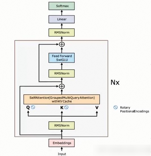
1.2 Transformers
1.2.1 Dense场景
通用场景中,transformers模型结构如下图示意,在计算model_flops时通常会考虑占比较大的模块例如qkv矩阵计算、self_atten、outout_linear等,而忽略占比较小的模块例如RMSNorm、Dropout、Softmax等。
Megatron-LM计算model_flops的函数如下所示:参考master-core0.12.x代码。分为3部分,分别是Attention、MLP、Logits。
1.2.1.1 Attention
计算公式:
分为两个部分,前者为基数部分,后者为计算部分。
(expansion_factor
        * batch_size
        * seq_length
        * num_layers
        * hidden_size
        * hidden_size ) ×(
                (
                    1                                                                               # 对应第1部分
                    + (num_query_groups / num_attention_heads)      # 对应第2部分
                    + (seq_length / hidden_size / 2)                              # 对应第3部分
                )
                * query_projection_to_hidden_size_ratio   # 通常是1
            )
过程分析:
self_attention计算也是分为3部分,分别是qkv_linear、core_attention、output_linear。其中第1、3部分都是linear,
- 第一部分:[S,B,H]×[H,H]—>[S,B,H],计算量为:SBHH。
- 第三部分:[S,B,H]×[H,H2]—>[S,B,H2],计算量为:S×B×H×H2。其中H表示hidden_size,h2受到GQA的影响,例如num_query_groups=8,num_attention_heads=64,则h2=1/8 * hidden_size,即h2=hidden_size÷num_attention_heads×num_query_groups。
- 第二部分:即core_attention,计算如下所示:
计算公式为
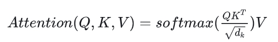 ,理论model_flops分析如下:(假设Q/K/V维度都是[BSH])
Q×Kt = [B,S,H][B,H,S]=[B,S,S],计算量为:BSHS
__softmax()V=[B,S,S]*[B,S,H]=[B,S,H],计算量为:BSSH。
上述两部分计算量之和为:2BSSH,考虑到caucal场景时atten_mask有一半为0,即不参与有效计算,因此理论计算量需要除以2,即计算量为:BSSH。
4. 合计:考虑到网络层数L,则合计总的计算次数=L×(SBHH+SBHH2+BSSH)=LSBHH×(1 + H2 + S/H),考虑到正反向、乘加运算以及FFN升降维运算,因此需要乘以一个基数expansion_factor,基数的含义如下所示:
# The 12x term below comes from the following factors; for more details, see
# "APPENDIX: FLOATING-POINT OPERATIONS" in https://arxiv.org/abs/2104.04473.
# - 3x: Each GEMM in the model needs to be performed 3 times (forward pass,
#    backward wgrad [weight gradient], backward dgrad [data gradient]).
# - 2x: GEMMs of a particular size are stacked twice in the standard Transformer model
#    architectures implemented in this codebase (e.g., h->ffn_h GEMM and ffn_h->h GEMM
#    in MLP layer).
# - 2x: A GEMM of a m*n tensor with a n*k tensor requires 2mnk floating-point operations.

expansion_factor = 3 * 2 * 2
注意:由于core_attention并不涉及GEMMs的升降维运算,因此其基数为6.
综上所述:Transformers的self attention模块的model_flops=12×LSBHH×(1 + H2 + S/H/2)。
1.2.1.2 MLP
计算公式:
(expansion_factor
        * batch_size
        * seq_length
        * num_layers
        * hidden_size
        * hidden_size ) × (
                (ffn_hidden_size / hidden_size)
                # * num_experts_routed_to
                * gated_linear_multiplier
            )
过程分析:
SBH*HF=SBF,计算量=SBHF=seq_length*batch_size*hidden_size*ffn_hidden_size。考虑swiglu激活函数,因此需要乘以gated_linear_multiplier(3/2)
SwiGLU(Swish-Gated Linear Unit)作为前馈网络(FFN)的激活函数时,其计算量是标准线性层的1.5倍(即3/2),因为SwiGLU需要执行两次线性变换(W1x和W2x)和一次逐元素乘法操作。
同上所述,考虑网络层数、正反向、乘加运算以及GEMM升降维度,设置expansion_factor基数为12。综上所述,MLP模块model_flops=12×LSBH×(F×gated_linear_multiplier)。
1.2.1.3 Logits
计算公式:
(expansion_factor
        * batch_size
        * seq_length
        * num_layers
        * hidden_size
        * hidden_size ) × (padded_vocab_size / (2 * num_layers * hidden_size)))
过程分析:
SBH×HV=SBV,计算量=SBHV=seq_length*batch_size*hidden_size*padded_vocab_size,expansion_factor是缩放因子,其默认值为12(3:正向+反向dx+反向yw; 2:乘加; 2:先上采样再下采样),但由于此处logits无下采样过程,因此缩放因子为6。综述所述,Logits模块model_flops=6×SBH×vocab_size。
1.2.2 MOE
MoE(Mixture of Experts)模型在计算model_flops时需要区分专家激活部分和非激活部分,仅前者需要参与计算model_flops。此外,MoE模型会引入门控网络和需要对专家输出进行融合,这两部分都可能会引入额外的flops计算量。
门控网络:
通常使用MLP+Softmax结构,对每个token计算E个专家得分,最后基于得分选择k个专家,计算逻辑为:(S,B,H) × (H,E)—>(S,B,E)。
易知model_flops=2×3×LSBHE=6LSBHE。
专家计算:
单个专家结构:Linear(H→F) → GELU → Linear(F→H),其中F常取值为4×hidden_size,根据上述MLP model_flops分析易知单个专家model_flops=12×LSBH×(F×gated_linear_multiplier)。
进而,k个专家model_flops=12k×LSBH×(F×gated_linear_multiplier)。
专家融合:
部分 MoE 会对 k 个专家的输出进行加权融合(权重来自门控网络的得分)
- 加权融合:每个输出维度需要k次乘法和k-1次加法,近似为:model_flops=2×3×k×LSBH=6kLSBH。
- 直接拼接融合:model_flops=0。
1.3 常见三方工具
1.3.1 Megatron-LM
Megatron-LM计算model_flops的函数如下所示:参考master-core0.12.x代码。分为3部分,分别是Attention、MLP、Logits:
def num_floating_point_operations():
    # Attention projection size.
    query_projection_size = kv_channels * num_attention_heads
    query_projection_to_hidden_size_ratio = query_projection_size / hidden_size
    # Group Query Attention.
    if not group_query_attention:
        num_query_groups = num_attention_heads
    else:
        num_query_groups = 8
    # MoE.
    # num_experts_routed_to = 1 if num_experts is None else moe_router_topk
    gated_linear_multiplier = 3 / 2 if swiglu else 1

    # The 12x term below comes from the following factors; for more details, see
    # "APPENDIX: FLOATING-POINT OPERATIONS" in https://arxiv.org/abs/2104.04473.
    # - 3x: Each GEMM in the model needs to be performed 3 times (forward pass,
    #       backward wgrad [weight gradient], backward dgrad [data gradient]).
    # - 2x: GEMMs of a particular size are stacked twice in the standard Transformer model
    #       architectures implemented in this codebase (e.g., h->ffn_h GEMM and ffn_h->h GEMM
    #       in MLP layer).
    # - 2x: A GEMM of a m*n tensor with a n*k tensor requires 2mnk floating-point operations.
    expansion_factor = 3 * 2 * 2

    return (
        expansion_factor
        * batch_size
        * seq_length
        * num_layers
        * hidden_size
        * hidden_size
        * (
            # Attention.
            (
                (
                    1
                    + (num_query_groups / num_attention_heads)
                    + (seq_length / hidden_size /2)
                ) * query_projection_to_hidden_size_ratio
            )
            # MLP.
            + (
                (ffn_hidden_size / hidden_size)
                #* num_experts_routed_to
                * gated_linear_multiplier
            )
            # Logit.
            + (padded_vocab_size / (2 * num_layers * hidden_size))
        )
    )
目前只支持Dense模型,还不支持MoE、MLA等场景。
1.3.2 DeepSpeed
该方法和如下介绍的PTA profiling方法有一定相似性,通过对例如:Torch的原生API进行Patch替换,实现准确的model_flops统计。和上述Megatron-LM方法存在区别,megatron不是在API级别进行flops计算,更多的是在mudole级别进行flops估计。
1.3.2.1 适用场景
类似于torch.profiling功能,支持在训推场景,DeepSpeed Runtime和非DeepSpeed场景使用,当前仅适用于Torch框架。 参考:Flops Profiler
1.3.2.2 使用方法
- DeepSpeed场景:(在ds_config.json配置文件中增加flops_profiler配置项)
{
  "flops_profiler": {
    "enabled": true,      # 使能开关
    "profile_step": 1,    # 采集步数
    "module_depth": -1,   # 采集模型层级(默认-1表示采集最内层级)
    "top_modules": 1,
    "detailed": true,
    "output_file": null
    }
}
- 非DeepSpeed场景:该场景使用内置的FlopsProfiler类对模型进行Wrap,即可在模型训练过程中通过start_profile、stop_profile、get_total_flops、get_total_macs、print_model_profile等实现功能启闭、信息采集、数据打印等功能。
from deepspeed.profiling.flops_profiler import FlopsProfiler

model = Model()
prof = FlopsProfiler(model)

profile_step = 5
print_profile= True

for step, batch in enumerate(data_loader):
  # start profiling at training step "profile_step"
  if step == profile_step:   # 开启flops profiling功能
    prof.start_profile()

  # forward() method
  loss = model(batch)

  # end profiling and print output
  if step == profile_step: # if using multi nodes, check global_rank == 0 as well   # 在特定步数采集flops数据并打印,结束flops profiling
    prof.stop_profile()
    flops = prof.get_total_flops()
    macs = prof.get_total_macs()
    params = prof.get_total_params()
    if print_profile:
        prof.print_model_profile(profile_step=profile_step)
    prof.end_profile()

  # runs backpropagation
  loss.backward()

  # weight update
  optimizer.step()
使用效果:打印模型切分信息、参数信息、MAC、FLPOS、正反向耗时等,打印网络层级、每层级参数量、MAC、时延、FLOPS等。
-------------------------- DeepSpeed Flops Profiler --------------------------
Profile Summary at step 10:
Notations:
data parallel size (dp_size), model parallel size(mp_size),
number of parameters (params), number of multiply-accumulate operations(MACs),
number of floating-point operations (flops), floating-point operations per second (FLOPS),
fwd latency (forward propagation latency), bwd latency (backward propagation latency),
step (weights update latency), iter latency (sum of fwd, bwd and step latency)

world size:                                                   1
data parallel size:                                           1
model parallel size:                                          1
batch size per GPU:                                           80
params per gpu:                                               336.23 M
params of model = params per GPU * mp_size:                   336.23 M
fwd MACs per GPU:                                             3139.93 G
fwd flops per GPU:                                            6279.86 G
fwd flops of model = fwd flops per GPU * mp_size:             6279.86 G
fwd latency:                                                  76.67 ms
bwd latency:                                                  108.02 ms
fwd FLOPS per GPU = fwd flops per GPU / fwd latency:          81.9 TFLOPS
bwd FLOPS per GPU = 2 * fwd flops per GPU / bwd latency:      116.27 TFLOPS
fwd+bwd FLOPS per GPU = 3 * fwd flops per GPU / (fwd+bwd latency):   102.0 TFLOPS
step latency:                                                 34.09 us
iter latency:                                                 184.73 ms
samples/second:                                               433.07

----------------------------- Aggregated Profile per GPU -----------------------------
Top modules in terms of params, MACs or fwd latency at different model depths:
depth 0:
    params      - {'BertForPreTrainingPreLN': '336.23 M'}
    MACs        - {'BertForPreTrainingPreLN': '3139.93 GMACs'}
    fwd latency - {'BertForPreTrainingPreLN': '76.39 ms'}
depth 1:
    params      - {'BertModel': '335.15 M', 'BertPreTrainingHeads': '32.34 M'}
    MACs        - {'BertModel': '3092.96 GMACs', 'BertPreTrainingHeads': '46.97 GMACs'}
    fwd latency - {'BertModel': '34.29 ms', 'BertPreTrainingHeads': '3.23 ms'}
depth 2:
    params      - {'BertEncoder': '302.31 M', 'BertLMPredictionHead': '32.34 M'}
    MACs        - {'BertEncoder': '3092.88 GMACs', 'BertLMPredictionHead': '46.97 GMACs'}
    fwd latency - {'BertEncoder': '33.45 ms', 'BertLMPredictionHead': '2.61 ms'}
depth 3:
    params      - {'ModuleList': '302.31 M', 'Embedding': '31.79 M', 'Linear': '31.26 M'}
    MACs        - {'ModuleList': '3092.88 GMACs', 'Linear': '36.23 GMACs'}
    fwd latency - {'ModuleList': '33.11 ms', 'BertPredictionHeadTransform': '1.83 ms''}
depth 4:
    params      - {'BertLayer': '302.31 M', 'LinearActivation': '1.05 M''}
    MACs        - {'BertLayer': '3092.88 GMACs', 'LinearActivation': '10.74 GMACs'}
    fwd latency - {'BertLayer': '33.11 ms', 'LinearActivation': '1.43 ms'}
depth 5:
    params      - {'BertAttention': '100.76 M', 'BertIntermediate': '100.76 M'}
    MACs        - {'BertAttention': '1031.3 GMACs', 'BertIntermediate': '1030.79 GMACs'}
    fwd latency - {'BertAttention': '19.83 ms', 'BertOutput': '4.38 ms'}
depth 6:
    params      - {'LinearActivation': '100.76 M', 'Linear': '100.69 M'}
    MACs        - {'LinearActivation': '1030.79 GMACs', 'Linear': '1030.79 GMACs'}
    fwd latency - {'BertSelfAttention': '16.29 ms', 'LinearActivation': '3.48 ms'}

------------------------------ Detailed Profile per GPU ------------------------------
Each module profile is listed after its name in the following order:
params, percentage of total params, MACs, percentage of total MACs, fwd latency, percentage of total fwd latency, fwd FLOPS

BertForPreTrainingPreLN(
  336.23 M, 100.00% Params, 3139.93 GMACs, 100.00% MACs, 76.39 ms, 100.00% latency, 82.21 TFLOPS,
  (bert): BertModel(
    335.15 M, 99.68% Params, 3092.96 GMACs, 98.50% MACs, 34.29 ms, 44.89% latency, 180.4 TFLOPS,
    (embeddings): BertEmbeddings(...)
    (encoder): BertEncoder(
      302.31 M, 89.91% Params, 3092.88 GMACs, 98.50% MACs, 33.45 ms, 43.79% latency, 184.93 TFLOPS,
      (FinalLayerNorm): FusedLayerNorm(...)
      (layer): ModuleList(
        302.31 M, 89.91% Params, 3092.88 GMACs, 98.50% MACs, 33.11 ms, 43.35% latency, 186.8 TFLOPS,
        (0): BertLayer(
          12.6 M, 3.75% Params, 128.87 GMACs, 4.10% MACs, 1.29 ms, 1.69% latency, 199.49 TFLOPS,
          (attention): BertAttention(
            4.2 M, 1.25% Params, 42.97 GMACs, 1.37% MACs, 833.75 us, 1.09% latency, 103.08 TFLOPS,
            (self): BertSelfAttention(
              3.15 M, 0.94% Params, 32.23 GMACs, 1.03% MACs, 699.04 us, 0.92% latency, 92.22 TFLOPS,
              (query): Linear(1.05 M, 0.31% Params, 10.74 GMACs, 0.34% MACs, 182.39 us, 0.24% latency, 117.74 TFLOPS,...)
              (key): Linear(1.05 M, 0.31% Params, 10.74 GMACs, 0.34% MACs, 57.22 us, 0.07% latency, 375.3 TFLOPS,...)
              (value): Linear(1.05 M, 0.31% Params, 10.74 GMACs, 0.34% MACs, 53.17 us, 0.07% latency, 403.91 TFLOPS,...)
              (dropout): Dropout(...)
              (softmax): Softmax(...)
            )
            (output): BertSelfOutput(
              1.05 M, 0.31% Params, 10.74 GMACs, 0.34% MACs, 114.68 us, 0.15% latency, 187.26 TFLOPS,
              (dense): Linear(1.05 M, 0.31% Params, 10.74 GMACs, 0.34% MACs, 64.13 us, 0.08% latency, 334.84 TFLOPS, ...)
              (dropout): Dropout(...)
            )
          )
          (PreAttentionLayerNorm): FusedLayerNorm(...)
          (PostAttentionLayerNorm): FusedLayerNorm(...)
          (intermediate): BertIntermediate(
            4.2 M, 1.25% Params, 42.95 GMACs, 1.37% MACs, 186.68 us, 0.24% latency, 460.14 TFLOPS,
            (dense_act): LinearActivation(4.2 M, 1.25% Params, 42.95 GMACs, 1.37% MACs, 175.0 us, 0.23% latency, 490.86 TFLOPS,...)
          )
          (output): BertOutput(
            4.2 M, 1.25% Params, 42.95 GMACs, 1.37% MACs, 116.83 us, 0.15% latency, 735.28 TFLOPS,
            (dense): Linear(4.2 M, 1.25% Params, 42.95 GMACs, 1.37% MACs, 65.57 us, 0.09% latency, 1310.14 TFLOPS,...)
            (dropout): Dropout(...)
          )
        )
        ...
        (23): BertLayer(...)
      )
    )
    (pooler): BertPooler(...)
  )
  (cls): BertPreTrainingHeads(...)
)
------------------------------------------------------------------------------
1.3.2.3 框架原理介绍
核心代码-文件组织结构:GitHub代码链接
deepspeed/profiling/flops_profiler/profiler.py
    get_model_profile
get_model_profile是总入口函数,实现profile实例的定义,包括系列核心工具类函数,如下图所示:
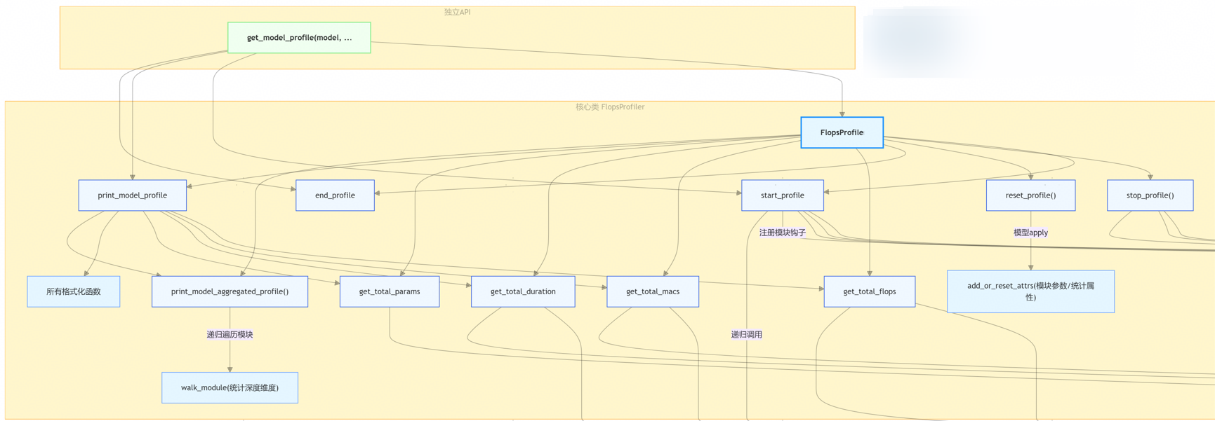
各个核心工具类:递归地进行数据采集,核心数据包括:模块耗时duration、乘加次数macs、model_flops等。
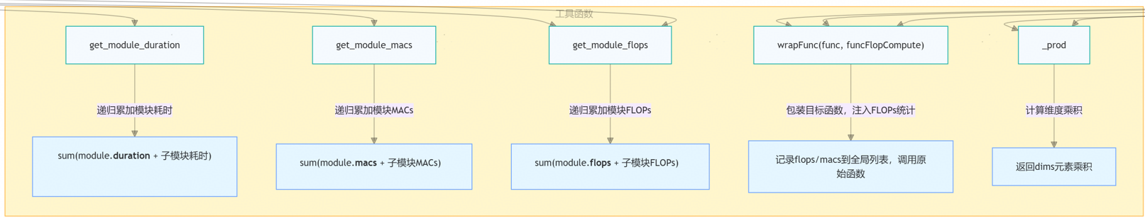
model_flops计算函数由如下系列函数构成:包括但不限于
\1. relu、elu、silu、gelu等激活函数组件、
\2. batch_norm、layer_norm、group_norm等Norm函数、
\3. gru、lstm、朴素rnn等RNN组件
\4. conv、pool、upsample等图像操作组件
\5. mul、addmm、matmul、linear、attention、softmax等组件
明细函数如下图所示:

1.3.3 torch_npu.profiling
1.3.3.1 适用场景
在某些场景,例如没有线程的model_flops计算代码、或者例如Pack数据模式下Megatron-LM原生的num_floating_point_operations计算函数失准,则可以通过torch_npu profiling的功能实现model_flops的准确计算。
不过注意点是,profiling数据采集过程耗时,无法像Megatron-LM在每个step自动快速计算model_flops,只能在特定步数采集获取model_flops信息,当模型结构、训练配置发生变化则需要重新采集,没有Megatron-LM那样便捷。
1.3.3.2 使用方法
例如在EOD场景/Pack数据模式下(不限于该场景),通过Megatron原生的num_floating_point_operations函数计算的model_flops失准,需要基于profiling采集model_flops。以MindSpeed-LLM为例,介绍如下步骤:
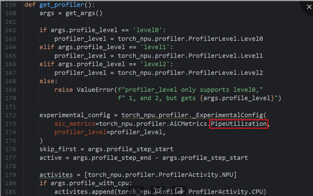
\1. 打开mindspeed_llm/training/training.py,找到get_profiler()方法,将PipeUtilization修改为ArithmeticUtilization
2、拉起训练,采集profiling。
3、打开采集的profiling中的 ASCEND_PROFILER_OUTPUT/kernel_details.csv 文件
4、把aic_cube_fops列求和,得到的结果就是model_flops;
MFU=modelflops/单卡峰值算力/迭代时间
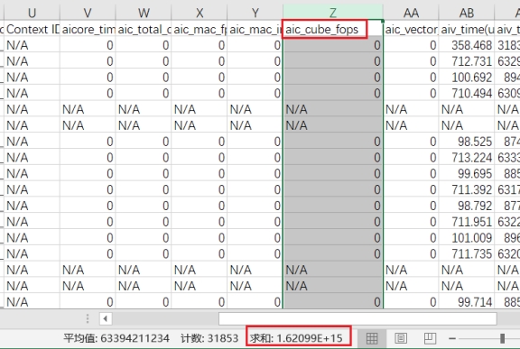
以上图为例,单步迭代时间为10.64s,单卡峰值算力为354TFlops,则MFU=(1.62099e+15)/(10e+12)/10.64/354=0.4304
1.4 其它三方工具
1.4.1 常见三方法介绍
calflops、ptflops、thop、torchstat、torchsumary、fvcore,以及使用方法
1.4.2 适用场景选择
| 三方库名 | 适用场景/特点 |
|---|---|
| torchstat | 不推荐,FLOPs和MACs概念搞反,不推荐。 |
| fvcore | 输出MACs,FLOPs和MACs混淆,不推荐。 |
| thop/ptflops | 输出MACs,需要将构造transformer模型输入的过程先处理好,然后再借助它们计算FLOPs的API提供的参数进行传入,形如: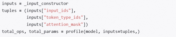 |
| calflops | 严格区分FLOPs和MACs,传入tokenizer作为transformer_tokenizer参数,形如: 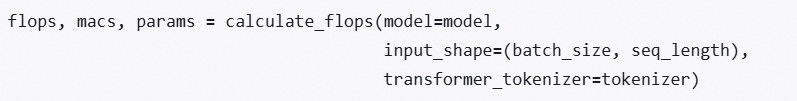 推荐的三方库,Github链接,计算的FLOPs计算相对准确,使用方式便捷,主要适用于transformers模型实现。 |
二、场景补充说明
2.1 部分参数冻结场景
模型在训练过程中有些场景可能会涉及模型参数冻结,包括但不限于Lora、多模态理解模型中的ViT冻结、强化学习中Ref参数冻结等。参数冻结对于MFU计算而言,意味着冻结参数对应的模块没有反向过程,因此不需要计算反向过程中的model flops。
- Lora场景:LoRA(Low-Rank Adaptation)是大模型高效微调的核心技术,核心思想是冻结主模型权重,仅通过低秩矩阵模拟权重更新,大幅降低微调的参数量和计算量。如下图:
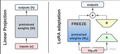
针对 Transformer 的注意力层(Query/Key/Value 投影矩阵,Q/K/V)或前馈网络(FFN),在原有权重矩阵 W ∈ R d × k W∈R^{d×k} W∈Rd×k旁,新增两个低秩矩阵: A ∈ R d × r A∈R^{d×r} A∈Rd×r:输入投影矩阵(随机初始化)
B ∈ R r × k B∈R^{r×k} B∈Rr×k:输出投影矩阵(初始化为 0); 其中 r 是低秩维度(通常取 8/16/32,远小于 d/k,如 d=4096 时 r=16)。
Lora场景,由于反向传播只需计算低秩矩阵的梯度,因此反向计算FLOPs骤降(前向FLOPs一般保持不变)。并且由于低秩矩阵参数量一般只占全部参数量的0.1%~1%,因此在某些对MFU计算精度要求并不很高的情况下,可能会忽略低秩的前反向过程。
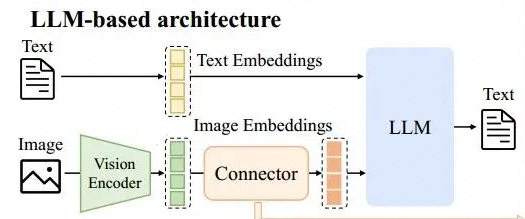
- 多模态理解模型场景:
当前多模态理解模型主流架构如下图所示:其中Vision Encoder(例如ViT)和Connector(VLAdapter,通常为MLP结构)通常为参数冻结状态,因此在计算model flops针对这些模块只计算前向过程。
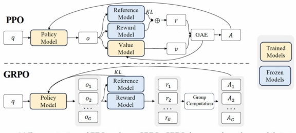
- GRPO REF模块:在RL场景,以去如下图GRPO算法为例,Ref参数模型和Rew奖励模型通常是冻结状态,因此在计算RL场景模型的model flops时也只需要考虑参数模型和奖励模型的前向。
2.2 关于有效计算量
在模型实际计算过程中可能会包含一些冗余计算,对于冗余计算是否需要加入到model flops中去,不同框架可能有不同的选择。
-
重计算场景:其中最明显的冗余计算属于重计算场景,硬件实际消耗了算力,但重计算通常是由于模型过大/显存较小而引入,将重计算引入的计算量加入到model flops中时所得到的MFU并不能和模型吞吐等价。因此Megatron-LM框架计算model flops时并没有考虑重计算的因素。
-
微调场景:在对大模型微调场景中,模型输入可能会被padding到最大序列长度,输入中padding的部分在计算Attention时实际也会参与计算,但padding的部分并不会影响模型的loss。
通常认为微调场景padding部分引入的计算和重计算都是属于无效计算量,这些部分是否要考虑到model flops中用于计算MFU,需要结合需求场景进行说明,同时这也可能会影响到目标MFU的确定。
2.3 变长序列场景
变长序列场景在Megatron-LM中对应–variable-seq-length配置,用于表示是否要对不同batch样本使用变长序列长度,使用该配置则不会引入padding以及对应的无效计算;不使用该配置则表示模型输入要被padding到最大序列长度。
在计算model_flops时,假如不考虑padding引入的冗余计算,由于实际训练样本的长度是非固定的,计算model flops时需要用到序列长度就需要通过平均值获取,而不能简单使用脚本中的--seq-length配置(否则会导致model flops偏高,而导致计算的MFU偏高)。

有“AI”的1024 = 2048,欢迎大家加入2048 AI社区
更多推荐


 8
8 0
0- 0


 已为社区贡献5条内容

所有评论(0)