（MATLAB版代码）红外与可见光图像配准算法 针对电气设备同一场景的红外与可见光图像间一致特征难以提取和匹配的问题，提出了一种基于斜率一致性的配准方法。 首先通过数学形态学方法分别提取红外与可见光图像的边缘，得到粗边缘图像；然后通过SURF算法提取两幅边缘图像的特征点，根据正确的匹配点对之间斜率一致性的先验知识，进行特征点匹配；最后通过最小二乘法求得仿射变换模型参数并实现两幅图像的配准。 资源为该算法的MATLAB版本，其中main.m是主函数，内附测试图片。

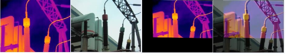
在处理电气设备同一场景的图像时，红外与可见光图像的配准一直是个让人头疼的问题，尤其是提取和匹配它们之间的一致特征，简直像在迷雾中找路。不过，今天咱就来唠唠一种基于斜率一致性的配准方法，而且还是MATLAB版本的哦！

一、整体思路

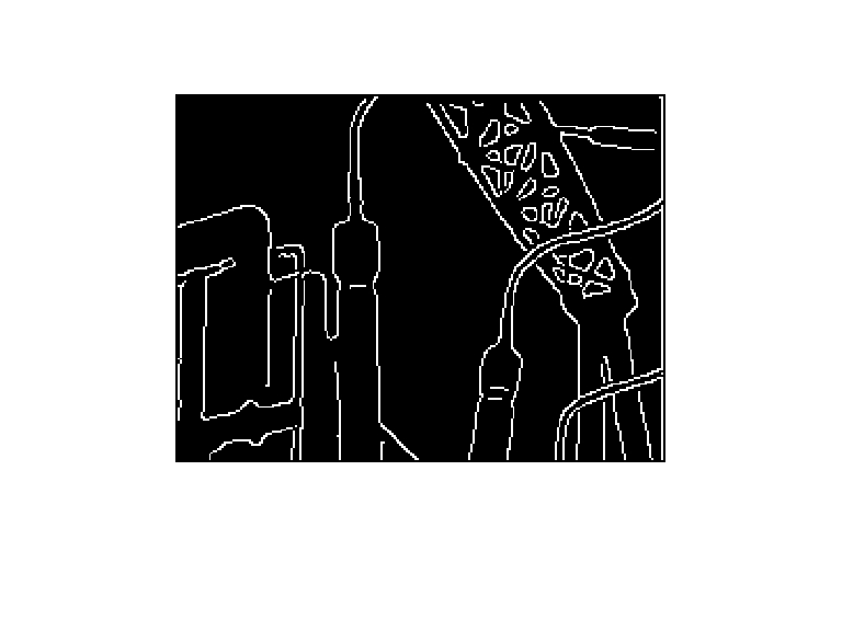
1. 边缘提取：利用数学形态学方法，分别从红外与可见光图像中提取边缘，获得粗边缘图像。这一步就像是给图像“描边”，把关键的轮廓先勾勒出来。
2. 特征点提取与匹配：借助SURF算法（加速稳健特征算法），在两幅边缘图像上找到特征点。然后，依据正确匹配点对之间斜率一致性这个先验知识，来进行特征点的匹配。就好比给这些特征点找到它们在另一幅图像中的“双胞胎”。
3. 图像配准：通过最小二乘法求出仿射变换模型的参数，最终实现两幅图像的配准，让它们完美“贴合”。

二、代码实现与分析

咱先看看 main.m 这个主函数（以下代码仅为示意，实际代码可能需根据具体需求调整）：

% main.m主函数
% 读取测试图片
irImage = imread('ir_test_image.jpg');
visImage = imread('vis_test_image.jpg');

% 边缘提取
se = strel('disk', 5); % 创建形态学结构元素
irEdge = imdilate(imbinarize(edge(irImage)), se); % 红外图像边缘提取
visEdge = imdilate(imbinarize(edge(visImage)), se); % 可见光图像边缘提取

% SURF特征点提取
pointsIR = detectSURFFeatures(irEdge);
pointsVIS = detectSURFFeatures(visEdge);
[featuresIR, validPointsIR] = extractFeatures(irEdge, pointsIR);
[featuresVIS, validPointsVIS] = extractFeatures(visEdge, pointsVIS);

% 特征点匹配
indexPairs = matchFeatures(featuresIR, featuresVIS);
matchedPointsIR = validPointsIR(indexPairs(:, 1), :);
matchedPointsVIS = validPointsVIS(indexPairs(:, 2), :);

% 斜率一致性筛选匹配点
correctMatches = [];
for i = 1:size(matchedPointsIR, 1)
    p1 = matchedPointsIR(i, :);
    p2 = matchedPointsVIS(i, :);
    % 这里简单示例斜率计算，实际可能需更复杂处理
    slope1 = (p1(2) - p1(1)) / (p1(4) - p1(3)); 
    slope2 = (p2(2) - p2(1)) / (p2(4) - p2(3)); 
    if abs(slope1 - slope2) < 0.1 % 设定斜率差值阈值
        correctMatches = [correctMatches; i];
    end
end
matchedPointsIR = matchedPointsIR(correctMatches, :);
matchedPointsVIS = matchedPointsVIS(correctMatches, :);

% 仿射变换模型参数计算与图像配准
tform = fitgeotrans(matchedPointsVIS, matchedPointsIR, 'affine');
registeredImage = imwarp(visImage, tform, 'OutputView', imref2d(size(irImage)));

% 显示结果
figure;
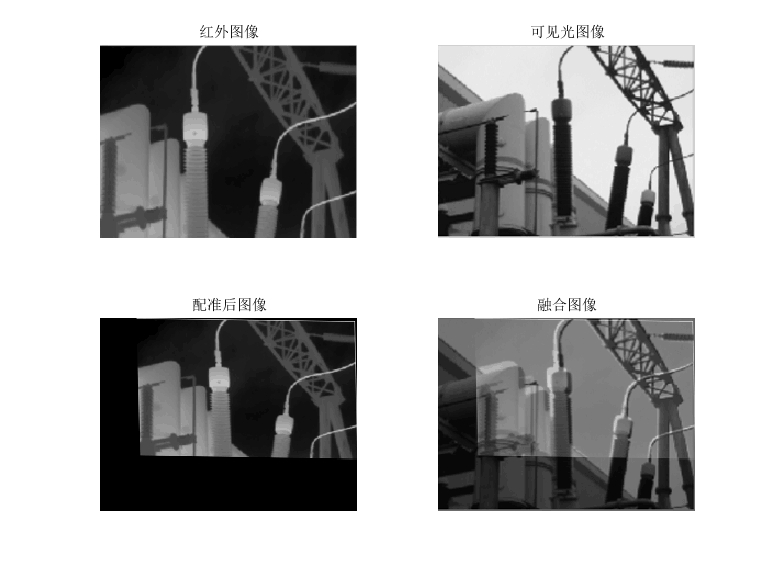
subplot(1, 3, 1); imshow(irImage); title('红外图像');
subplot(1, 3, 2); imshow(visImage); title('可见光图像');
subplot(1, 3, 3); imshow(registeredImage); title('配准后的可见光图像');

1. 读取测试图片

irImage = imread('ir_test_image.jpg');
visImage = imread('vis_test_image.jpg');

这部分没啥好说的，就是把红外和可见光的测试图片读进来，准备后续处理。就像先把食材准备好，才能下锅做菜嘛。

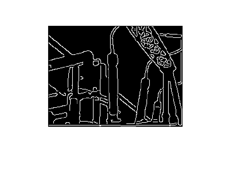
2. 边缘提取

se = strel('disk', 5); 
irEdge = imdilate(imbinarize(edge(irImage)), se); 
visEdge = imdilate(imbinarize(edge(visImage)), se); 

这里创建了一个半径为5的圆盘形结构元素 se，用来对图像进行形态学膨胀操作。先通过 edge 函数提取边缘，再 imbinarize 二值化，最后 imdilate 膨胀。这就好比给边缘“加粗”，让边缘特征更明显，便于后续特征点提取。

3. SURF特征点提取

pointsIR = detectSURFFeatures(irEdge);
pointsVIS = detectSURFFeatures(visEdge);
[featuresIR, validPointsIR] = extractFeatures(irEdge, pointsIR);
[featuresVIS, validPointsVIS] = extractFeatures(visEdge, pointsVIS);

detectSURFFeatures 函数用来检测图像中的SURF特征点，然后 extractFeatures 函数提取这些特征点对应的特征描述符。就像是给每个特征点贴上一个独特的“标签”，方便后续匹配。

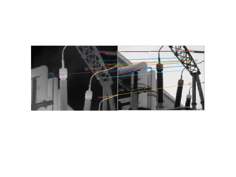
4. 特征点匹配

indexPairs = matchFeatures(featuresIR, featuresVIS);
matchedPointsIR = validPointsIR(indexPairs(:, 1), :);
matchedPointsVIS = validPointsVIS(indexPairs(:, 2), :);

matchFeatures 函数根据特征描述符找到可能匹配的点对，返回匹配点对的索引 indexPairs，然后根据索引得到实际的匹配点 matchedPointsIR 和 matchedPointsVIS。这一步就像是在茫茫“点海”中给每个点找“对象”。

5. 斜率一致性筛选匹配点

correctMatches = [];
for i = 1:size(matchedPointsIR, 1)
    p1 = matchedPointsIR(i, :);
    p2 = matchedPointsVIS(i, :);
    slope1 = (p1(2) - p1(1)) / (p1(4) - p1(3)); 
    slope2 = (p2(2) - p2(1)) / (p2(4) - p2(3)); 
    if abs(slope1 - slope2) < 0.1 
        correctMatches = [correctMatches; i];
    end
end
matchedPointsIR = matchedPointsIR(correctMatches, :);
matchedPointsVIS = matchedPointsVIS(correctMatches, :);

这部分代码遍历所有匹配点对，计算每对匹配点的斜率（这里只是简单示例计算方式），如果斜率差值小于设定阈值（这里设为0.1），就认为是正确匹配点，添加到 correctMatches 中。最后根据正确匹配点索引重新获取匹配点，这就把那些“不靠谱”的匹配点给筛掉了。

6. 仿射变换模型参数计算与图像配准

tform = fitgeotrans(matchedPointsVIS, matchedPointsIR, 'affine');
registeredImage = imwarp(visImage, tform, 'OutputView', imref2d(size(irImage)));

fitgeotrans 函数根据正确匹配点对计算仿射变换模型参数 tform，然后 imwarp 函数利用这个变换模型对可见光图像进行变换，得到配准后的图像 registeredImage。这就像是给可见光图像做了个“整形手术”，让它和红外图像完美对齐。

7. 显示结果

figure;
subplot(1, 3, 1); imshow(irImage); title('红外图像');
subplot(1, 3, 2); imshow(visImage); title('可见光图像');
subplot(1, 3, 3); imshow(registeredImage); title('配准后的可见光图像');

最后，把红外图像、可见光图像以及配准后的可见光图像一起显示出来，方便直观对比。就像把“手术”前后的照片摆在一起，看看效果咋样。

通过这种基于斜率一致性的配准方法，利用MATLAB实现起来还是挺有意思的。大家可以自己动手试试，说不定还能发现更好的优化方式呢！