视觉基础实战:分类检测+目标检测+语义分割+实例分割(CNN+YOLOV11+MMSegmentation)
视觉人工智能(Visual AI)作为计算机科学领域的重要分支,近年来取得了突飞猛进的发展。从简单的图像分类到复杂的目标检测和语义分割,视觉AI技术正在广泛应用于自动驾驶、医疗影像分析、工业质检、安防监控等众多领域。随着深度学习技术的不断演进,特别是卷积神经网络Transformer架构以及多模态大模型的兴起,视觉AI的性能和效率得到了显著提升。
三、MMSegmentation语义分割(PSPNet+DeepLab)
前言
视觉人工智能(Visual AI)作为计算机科学领域的重要分支,近年来取得了突飞猛进的发展。从简单的图像分类到复杂的目标检测和语义分割,视觉AI技术正在广泛应用于自动驾驶、医疗影像分析、工业质检、安防监控等众多领域。随着深度学习技术的不断演进,特别是卷积神经网络、Transformer架构以及多模态大模型的兴起,视觉AI的性能和效率得到了显著提升。本文通过三个具体的工程实践案例——CNN图像分类、YOLOv11目标检测和MMSegmentation语义分割,系统总结了视觉AI的关键技术路线和实现方法,旨在为相关领域的学习者和研究者提供实用的参考指南。从技术发展脉络来看,视觉AI正经历着从专用小模型到通用大模型的演进过程。如中国科学院自动化研究所紫东太初大模型研究中心指出,传统的视觉模型往往依赖于大量标注数据、泛化能力差,难以适应不同场景,而视觉基础模型通过自监督预训练和大规模参数学习,正逐步克服这些局限性。接下来的章节将详细阐述三种典型视觉任务的工程实践,并结合最新研究进展分析其技术原理与发展趋势。
一、CNN分类CIFAR-10
1.数据集准备
数据集可以在网址 https://www.cs.toronto.edu/~kriz/cifar.html 中进行下载
2.环境配置
conda create -n cnn python=3.8
conda activate cnn
根据自己的显卡型号,驱动版本,源码版本等进行选择pytorch
conda install pytorch torchvision torchaudio pytorch-cuda=12.1 -c pytorch -c nvidia
3.回到CNN检测(基于pytorch手搓)
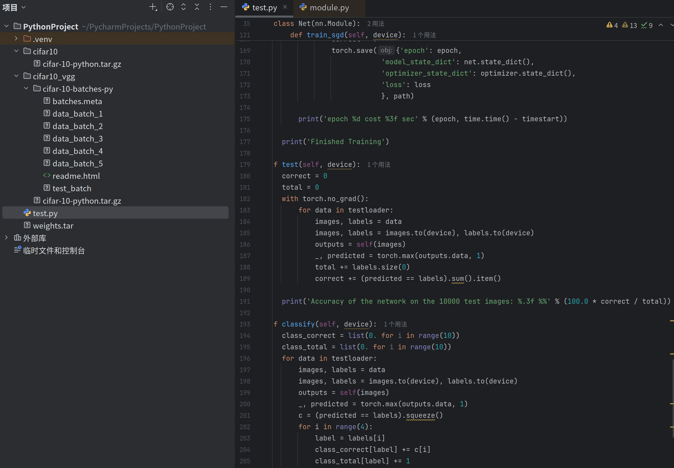
项目目录如下
#  声明:本代码并非自己编写,由他人提供
import torch
import torch.nn as nn
import torch.nn.functional as F
import torchvision
import torchvision.transforms as transforms
import torch.optim as optim
import time
import os
import ssl

ssl._create_default_https_context = ssl._create_unverified_context

transform = transforms.Compose(
    [
        transforms.RandomHorizontalFlip(),
        transforms.RandomGrayscale(),
        transforms.ToTensor(),
        transforms.Normalize((0.5, 0.5, 0.5), (0.5, 0.5, 0.5))])

transform1 = transforms.Compose(
    [
        transforms.ToTensor(),
        transforms.Normalize((0.5, 0.5, 0.5), (0.5, 0.5, 0.5))])

trainset = torchvision.datasets.CIFAR10(root='./cifar10_vgg', train=True, download=True, transform=transform)
trainloader = torch.utils.data.DataLoader(trainset, batch_size=100, shuffle=True, num_workers=2)

testset = torchvision.datasets.CIFAR10(root='./cifar10_vgg', train=False, download=True, transform=transform1)
testloader = torch.utils.data.DataLoader(testset, batch_size=50, shuffle=False, num_workers=2)

classes = ('plane', 'car', 'bird', 'cat', 'deer', 'dog', 'frog', 'horse', 'ship', 'truck')


class Net(nn.Module):

    def __init__(self):
        super(Net, self).__init__()
        self.conv1 = nn.Conv2d(3, 64, 3, padding=1)
        self.conv2 = nn.Conv2d(64, 64, 3, padding=1)
        self.pool1 = nn.MaxPool2d(2, 2)
        self.bn1 = nn.BatchNorm2d(64)
        self.relu1 = nn.ReLU()

        self.conv3 = nn.Conv2d(64, 128, 3, padding=1)
        self.conv4 = nn.Conv2d(128, 128, 3, padding=1)
        self.pool2 = nn.MaxPool2d(2, 2, padding=1)
        self.bn2 = nn.BatchNorm2d(128)
        self.relu2 = nn.ReLU()

        self.conv5 = nn.Conv2d(128, 128, 3, padding=1)
        self.conv6 = nn.Conv2d(128, 128, 3, padding=1)
        self.conv7 = nn.Conv2d(128, 128, 1, padding=1)
        self.pool3 = nn.MaxPool2d(2, 2, padding=1)
        self.bn3 = nn.BatchNorm2d(128)
        self.relu3 = nn.ReLU()

        self.conv8 = nn.Conv2d(128, 256, 3, padding=1)
        self.conv9 = nn.Conv2d(256, 256, 3, padding=1)
        self.conv10 = nn.Conv2d(256, 256, 1, padding=1)
        self.pool4 = nn.MaxPool2d(2, 2, padding=1)
        self.bn4 = nn.BatchNorm2d(256)
        self.relu4 = nn.ReLU()

        self.conv11 = nn.Conv2d(256, 512, 3, padding=1)
        self.conv12 = nn.Conv2d(512, 512, 3, padding=1)
        self.conv13 = nn.Conv2d(512, 512, 1, padding=1)
        self.pool5 = nn.MaxPool2d(2, 2, padding=1)
        self.bn5 = nn.BatchNorm2d(512)
        self.relu5 = nn.ReLU()

        self.fc14 = nn.Linear(512 * 4 * 4, 1024)
        self.drop1 = nn.Dropout2d()
        self.fc15 = nn.Linear(1024, 1024)
        self.drop2 = nn.Dropout2d()
        self.fc16 = nn.Linear(1024, 10)

    def forward(self, x):
        x = self.conv1(x)
        x = self.conv2(x)
        x = self.pool1(x)
        x = self.bn1(x)
        x = self.relu1(x)

        x = self.conv3(x)
        x = self.conv4(x)
        x = self.pool2(x)
        x = self.bn2(x)
        x = self.relu2(x)

        x = self.conv5(x)
        x = self.conv6(x)
        x = self.conv7(x)
        x = self.pool3(x)
        x = self.bn3(x)
        x = self.relu3(x)

        x = self.conv8(x)
        x = self.conv9(x)
        x = self.conv10(x)
        x = self.pool4(x)
        x = self.bn4(x)
        x = self.relu4(x)

        x = self.conv11(x)
        x = self.conv12(x)
        x = self.conv13(x)
        x = self.pool5(x)
        x = self.bn5(x)
        x = self.relu5(x)
        # print(" x shape ",x.size())
        x = x.view(-1, 512 * 4 * 4)
        x = F.relu(self.fc14(x))
        x = self.drop1(x)
        x = F.relu(self.fc15(x))
        x = self.drop2(x)
        x = self.fc16(x)

        return x

    def train_sgd(self, device):

        optimizer = optim.SGD(self.parameters(), lr=0.01)
        path = 'weights.tar'
        initepoch = 0

        if os.path.exists(path) is not True:
            loss = nn.CrossEntropyLoss()


        else:
            checkpoint = torch.load(path)
            self.load_state_dict(checkpoint['model_state_dict'])
            optimizer.load_state_dict(checkpoint['optimizer_state_dict'])
            initepoch = checkpoint['epoch']
            loss = checkpoint['loss']

        for epoch in range(initepoch, 20):  # loop over the dataset multiple times
            timestart = time.time()

            running_loss = 0.0
            total = 0
            correct = 0
            for i, data in enumerate(trainloader, 0):
                # get the inputs
                inputs, labels = data
                inputs, labels = inputs.to(device), labels.to(device)

                optimizer.zero_grad()

                outputs = self(inputs)
                l = loss(outputs, labels)
                l.backward()
                optimizer.step()

                running_loss += l.item()

                if i % 500 == 499:
                    print('[%d, %5d] loss: %.4f' %
                          (epoch, i, running_loss / 500))
                    running_loss = 0.0
                    _, predicted = torch.max(outputs.data, 1)
                    total += labels.size(0)
                    correct += (predicted == labels).sum().item()
                    print('Accuracy of the network on the %d tran images: %.3f %%' % (total,
                                                                                      100.0 * correct / total))
                    total = 0
                    correct = 0
                    torch.save({'epoch': epoch,
                                'model_state_dict': net.state_dict(),
                                'optimizer_state_dict': optimizer.state_dict(),
                                'loss': loss
                                }, path)

            print('epoch %d cost %3f sec' % (epoch, time.time() - timestart))

        print('Finished Training')

    def test(self, device):
        correct = 0
        total = 0
        with torch.no_grad():
            for data in testloader:
                images, labels = data
                images, labels = images.to(device), labels.to(device)
                outputs = self(images)
                _, predicted = torch.max(outputs.data, 1)
                total += labels.size(0)
                correct += (predicted == labels).sum().item()

        print('Accuracy of the network on the 10000 test images: %.3f %%' % (100.0 * correct / total))

    def classify(self, device):
        class_correct = list(0. for i in range(10))
        class_total = list(0. for i in range(10))
        for data in testloader:
            images, labels = data
            images, labels = images.to(device), labels.to(device)
            outputs = self(images)
            _, predicted = torch.max(outputs.data, 1)
            c = (predicted == labels).squeeze()
            for i in range(4):
                label = labels[i]
                class_correct[label] += c[i]
                class_total[label] += 1

        for i in range(10):
            print('Accuracy of %5s : %2d %%' % (classes[i], 100 * class_correct[i] / class_total[i]))


if __name__ == '__main__':
    device = torch.device("cuda:0" if torch.cuda.is_available() else "cpu")
    net = Net()
    net = net.to(device)
    net.train_sgd(device)
    net.test(device)
    net.classify(device)
4.运行结果
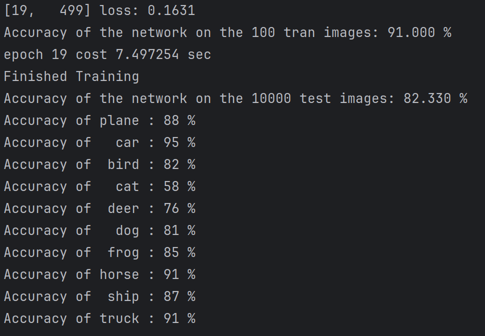
4.总结
此阶段主要熟悉数据集使用 以及通过代码学习:
网络架构:采用VGG风格的卷积神经网络,通过堆叠3×3卷积和最大池化层逐步提取特征,使用批归一化加速训练,Dropout防止过拟合
训练流程:实现了数据增强、模型训练、检查点保存与恢复。每500个batch输出损失和准确率,支持从断点继续训练。
工程实践:包含GPU自动检测、多进程数据加载、SSL证书处理等实用技巧。测试时使用torch.no_grad()节省内存,并提供整体和分类别准确率评估。
二、YOLOv11训练自己的数据集进行目标检测
1.环境配置
( 参考https://github.com/ultralytics/ultralytics )
官网下载好项目后配置环境
conda create -n yolov11 python=3.8

conda activate yolov11

pip install torch==2.0.0+cu118 torchvision==0.15.1+cu118 --extra-index-url https://download.pytorch.org/whl/cu118
(也可以通过下载好的whl文件直接安装torch等)
pip install torch-2.0.0+cu118-cp39-cp39-win_amd64.whl

安装ultralytics库
pip install ultralytics
可通过以下代码测试环境配置是否成功
from ultralytics import YOLO
# 加载预训练的 YOLOv11n 模型
model = YOLO('/home/hy/ultralytics/runs/detect/train5/weights/best.pt')
source = '/home/hy/ultralytics/img.png' #更改为自己的图片路径
# 运行推理,并附加参数
model.predict(source, save=True)
可在run/detect看到测试结果

2.数据集
https://universe.roboflow.com/
该网址非常适合获取目标检测数据集,文件标注格式齐全
在搜索框搜Safety helmet(本次实验针对安全帽做检测)
注册后,进入左侧栏目dataset点击右侧Download Dataset下载
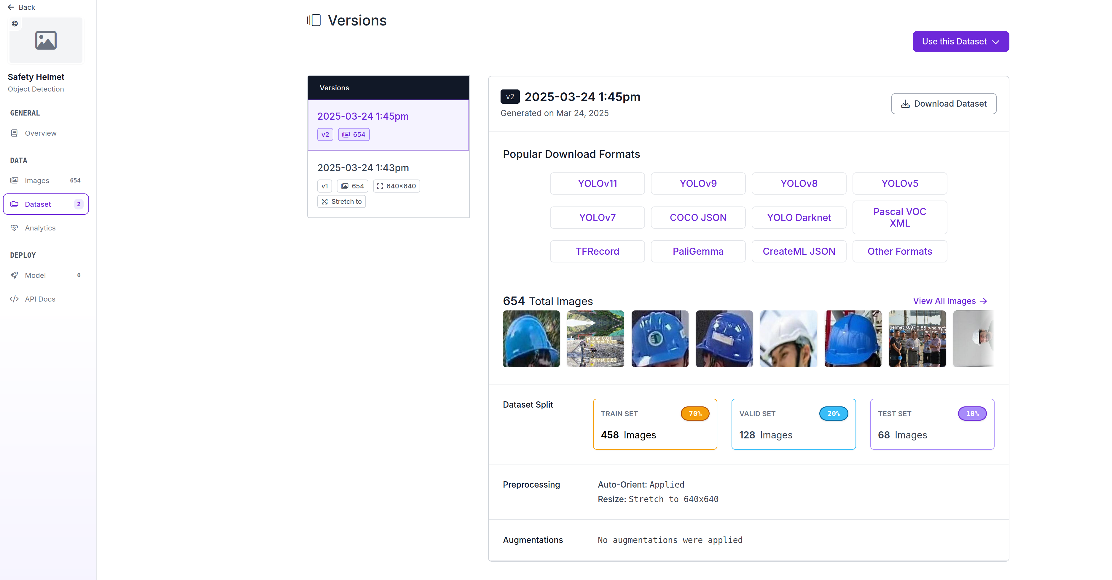
如下图选择yolo11格式(TXT)
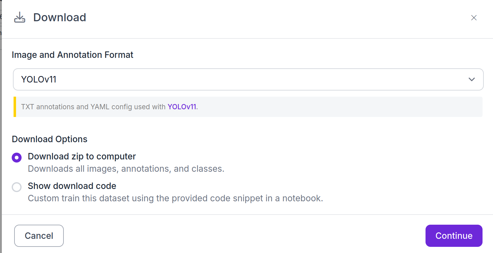
解压后就是训练所需的格式
3. 训练模型
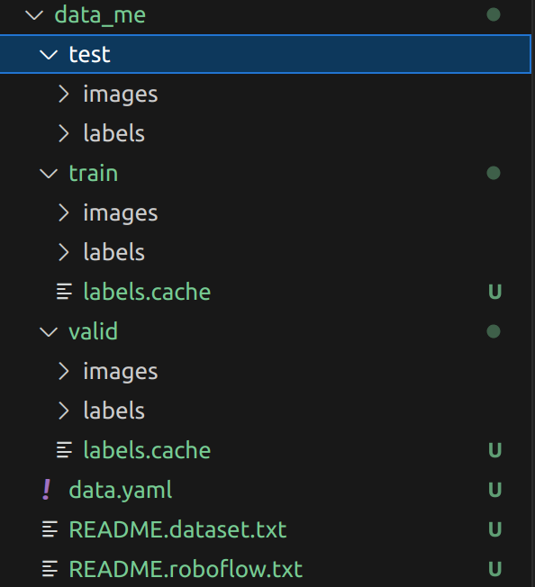
3.1 创建data.yaml
在yolov11根目录下(即本文所用的ultralytics目录下)创建一个新的data.yaml文件,也可以是其他名字的例如hat.yaml文件,文件名可以变但是后缀需要为.yaml,内容如下
train: /home/hy/ultralytics/data_me/train/images
val: /home/hy/ultralytics/data_me/valid/images
test: /home/hy/ultralytics/data_me/test/images

nc: 1
names: ['helmet']

roboflow:
  workspace: i-gusti-fajar
  project: safety-helmet-1nzb5
  version: 2
  license: CC BY 4.0
  url: https://universe.roboflow.com/i-gusti-fajar/safety-helmet-1nzb5/dataset/2
其他路径和类别自己替换,需要和上面数据集转换那里类别顺序一致。
3.2 训练模型
下载预训练权重进行训练,这里使用yolov11n.pt
ultralytics根目录中,创建一个yolov11_train.py文件,内容如下,关闭amp训练。没有GPU需要改 device="cpu" 。
import warnings
warnings.filterwarnings('ignore')
from ultralytics import YOLO
if __name__ == '__main__':
model = YOLO('ultralytics/cfg/models/11/yolo11n.yaml')
model.load('yolo11n.pt') #注释则不加载
results = model.train(
data='hat.yaml', #数据集配置文件的路径
epochs=200, #训练轮次总数
batch=16, #批量大小,即单次输入多少图片训练
imgsz=640, #训练图像尺寸
workers=8, #加载数据的工作线程数
device= 0, #指定训练的计算设备,无nvidia显卡则改为 'cpu'
optimizer='SGD', #训练使用优化器,可选 auto,SGD,Adam,AdamW 等
amp= True, #True 或者 False, 解释为:自动混合精度(AMP) 训练
cache=False # True 在内存中缓存数据集图像,服务器推荐开启
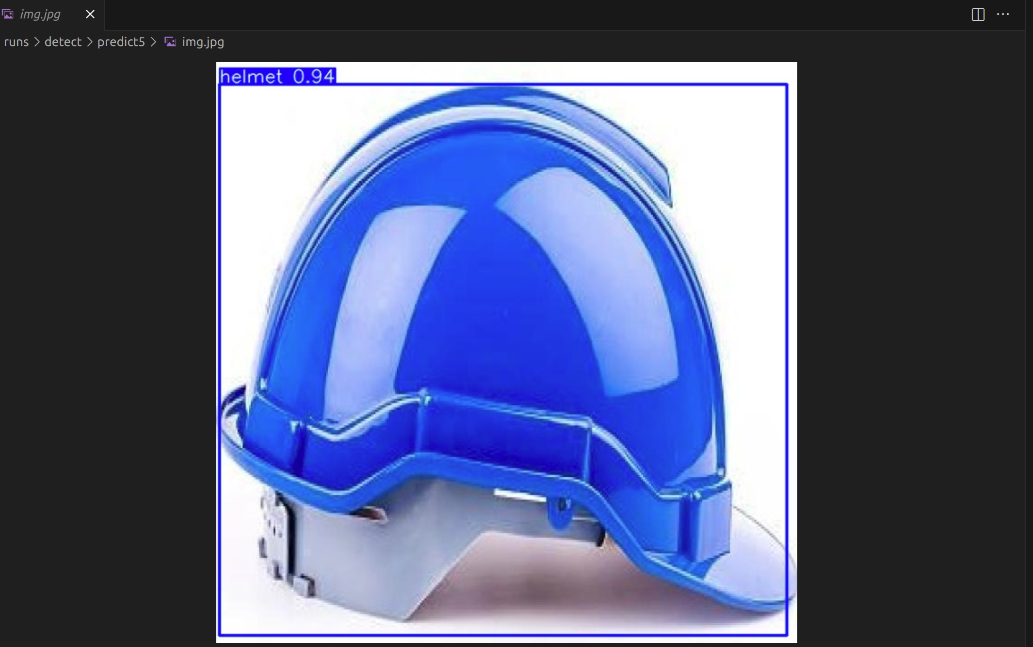
)4. 模型测试
找到之前训练的结果保存路径,创建一个yolov11_predict.py文件,内容如下
from ultralytics import YOLO
# 加载预训练的 YOLOv11n 模型
model = YOLO('/home/hy/ultralytics/runs/detect/train5/weights/best.pt')
source = '/home/hy/ultralytics/img.png' #更改为自己的图片路径
# 运行推理,并附加参数
model.predict(source, save=True)
运行后就会得到预测模型结果。
可在runs目录下看到结果
三、MMSegmentation语义分割(PSPNet+DeepLab)
1. mmseg安装
可参照官方文档进行安装https://mmsegmentation.readthedocs.io/zh-cn/latest/get_started.html
conda create --name openmmlab python=3.8 -y
conda activate openmmlab

在 GPU 平台上:

conda install pytorch torchvision -c pytorch

在 CPU 平台上

conda install pytorch torchvision cpuonly -c pytorch

步骤 0. 使用 MIM 安装 MMCV

pip install -U openmim
mim install mmengine
mim install "mmcv>=2.0.0"

步骤 1. 安装 MMSegmentation

情况 a: 如果您想立刻开发和运行 mmsegmentation,您可通过源码安装:

git clone -b main https://github.com/open-mmlab/mmsegmentation.git
cd mmsegmentation
pip install -v -e .
# '-v' 表示详细模式,更多的输出
# '-e' 表示以可编辑模式安装工程,
# 因此对代码所做的任何修改都生效,无需重新安装
验证安装是否成功
为了验证 MMSegmentation 是否正确安装,我们提供了一些示例代码来运行一个推理 demo 。
步骤 1. 下载配置文件和模型文件
mim download mmsegmentation --config pspnet_r50-d8_4xb2-40k_cityscapes-512x1024 --dest .
下载结束,您将看到以下两个文件在当前工作目录:pspnet_r50-d8_4xb2-40k_cityscapes-512x1024.py 和 pspnet_r50-d8_512x1024_40k_cityscapes_20200605_003338-2966598c.pth
步骤 2. 验证推理 demo
运行以下命令即可:
python demo/image_demo.py demo/demo.png configs/pspnet/pspnet_r50-d8_4xb2-40k_cityscapes-512x1024.py pspnet_r50-d8_512x1024_40k_cityscapes_20200605_003338-2966598c.pth --device cuda:0 --out-file result.jpg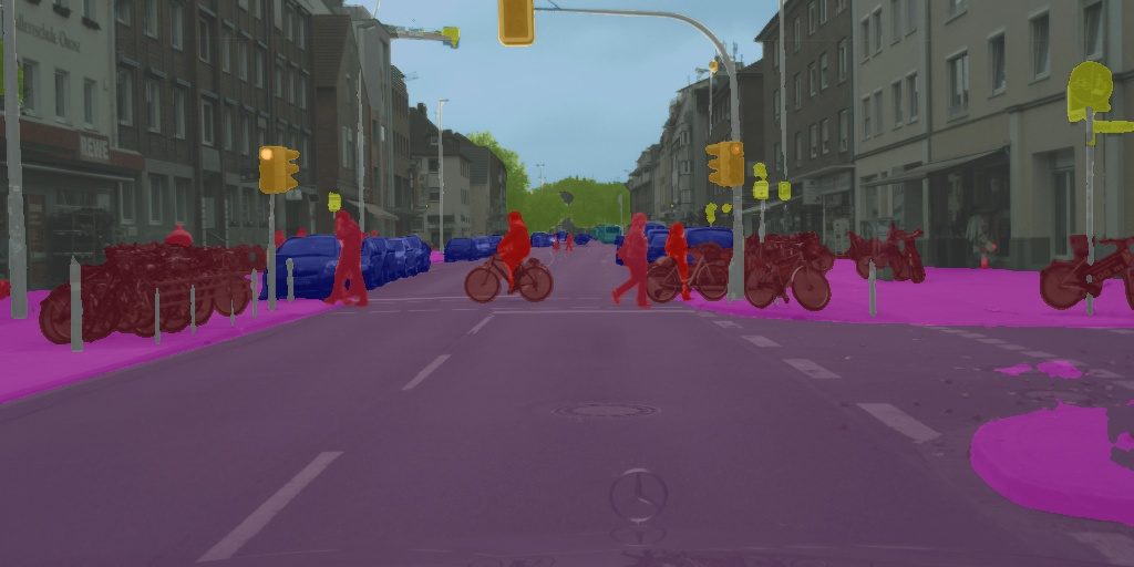
2. 数据集下载
进入cityscapes官网:https://www.cityscapes-dataset.com/downloads/
下载数据集需要用教育邮箱注册账号,我们注册并登录后下载这三个数据集:
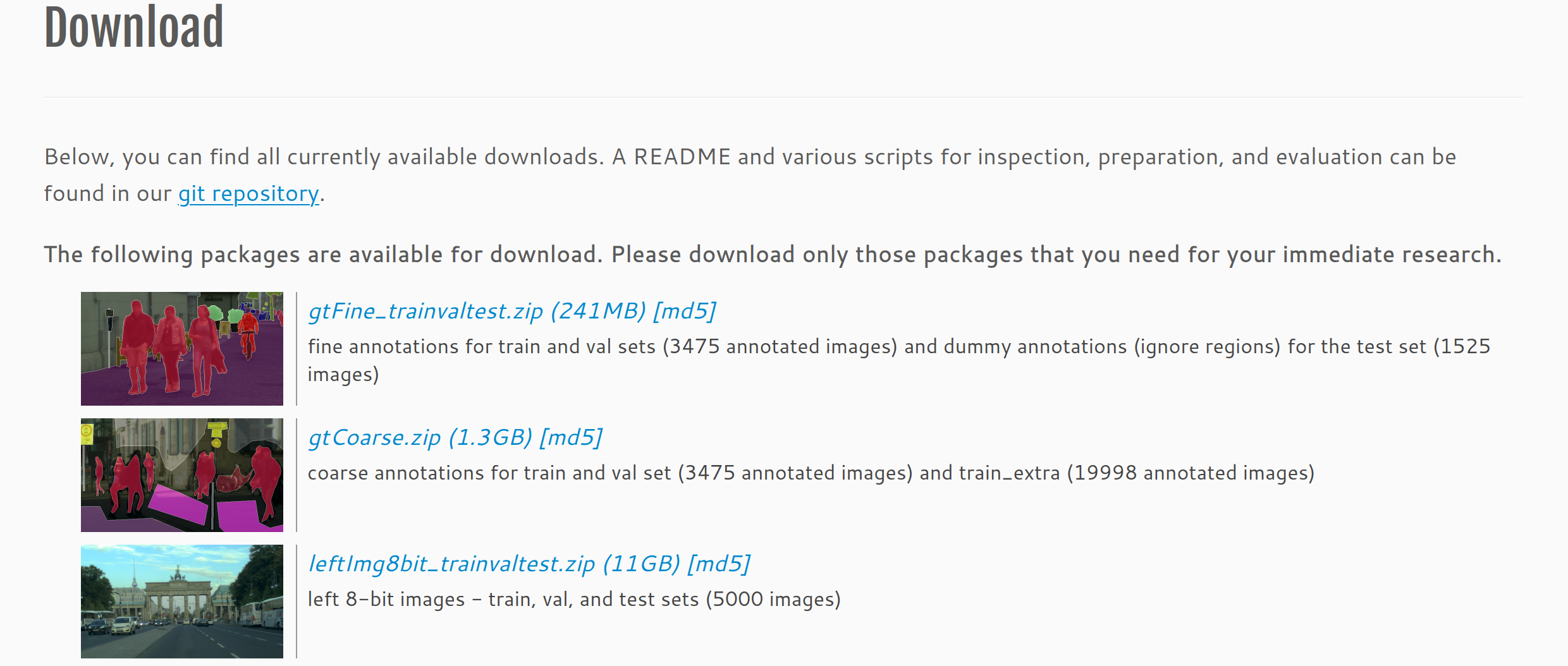
3. 数据集准备
在数据集下载完成后,我们需使用cityscapes数据集官方公开工具集创建带有标签ID的png图像工具集github地址 https://link.gitcode.com/i/bf6a551ba70e69925e33f6156cedbe8e?isLogin=1
下载cityscapesscripts后将其放置data目录
我们主要使用其中的preparation/createTrainIdLabelImgs.py,
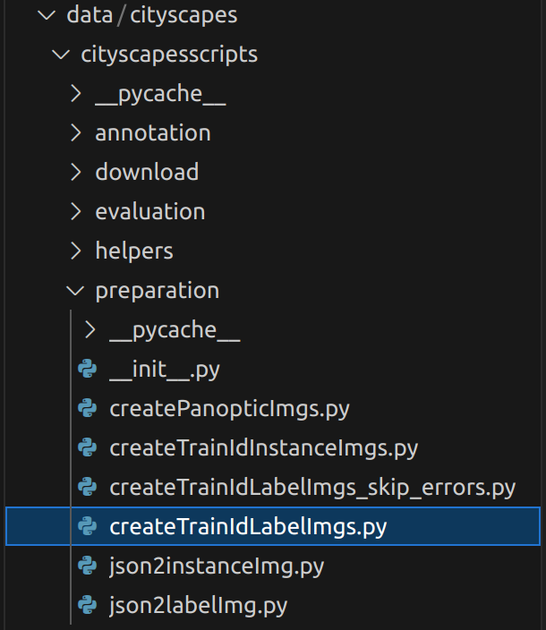
注意将cityscapesPath改为自己数据集的路径
#!/usr/bin/python
#
# Converts the polygonal annotations of the Cityscapes dataset
# to images, where pixel values encode ground truth classes.
#
# The Cityscapes downloads already include such images
#   a) *color.png             : the class is encoded by its color
#   b) *labelIds.png          : the class is encoded by its ID
#   c) *instanceIds.png       : the class and the instance are encoded by an instance ID
#
# With this tool, you can generate option
#   d) *labelTrainIds.png     : the class is encoded by its training ID
# This encoding might come handy for training purposes. You can use
# the file labels.py to define the training IDs that suit your needs.
# Note however, that once you submit or evaluate results, the regular
# IDs are needed.
#
# Uses the converter tool in 'json2labelImg.py'
# Uses the mapping defined in 'labels.py'
#

# python imports
from __future__ import print_function, absolute_import, division
import os, glob, sys

sys.path.append('/home/hy/mmsegmentation-main/data/cityscapes/cityscapesscripts')

# cityscapes imports
from cityscapesscripts.helpers.csHelpers import printError
from cityscapesscripts.preparation.json2labelImg import json2labelImg

# The main method
def main():
    # Where to look for Cityscapes
    # if 'CITYSCAPES_DATASET' in os.environ:
    #     cityscapesPath = os.environ['/home/hy/mmsegmentation-main/data/cityscapes']
    # else:
    #     cityscapesPath = os.path.join(os.path.dirname(os.path.realpath(__file__)),'..','..')
    # how to search for all ground truth
    cityscapesPath = os.environ['CITYSCAPES_DATASET']
    searchFine   = os.path.join( cityscapesPath , "gtFine"   , "*" , "*" , "*_gt*_polygons.json" )
    searchCoarse = os.path.join( cityscapesPath , "gtCoarse" , "*" , "*" , "*_gt*_polygons.json" )

    # search files
    filesFine = glob.glob( searchFine )
    filesFine.sort()
    filesCoarse = glob.glob( searchCoarse )
    filesCoarse.sort()

    # concatenate fine and coarse
    files = filesFine + filesCoarse
    # files = filesFine # use this line if fine is enough for now.

    # quit if we did not find anything
    if not files:
        printError( "Did not find any files. Please consult the README." )

    # a bit verbose
    print("Processing {} annotation files".format(len(files)))

    # iterate through files
    progress = 0
    print("Progress: {:>3} %".format( progress * 100 / len(files) ), end=' ')
    for f in files:
        # create the output filename
        dst = f.replace( "_polygons.json" , "_labelTrainIds.png" )

        # do the conversion
        try:
            json2labelImg( f , dst , "trainIds" )
        except:
            print("Failed to convert: {}".format(f))
            raise

        # status
        progress += 1
        print("\rProgress: {:>3} %".format( progress * 100 / len(files) ), end=' ')
        sys.stdout.flush()


# call the main
if __name__ == "__main__":
    main()
注意 此处应将CITYSCAPES_DATASET填为自己的路径
或设置环境变量export CITYSCAPES_DATASET=/path/to/your/cityscapes
在代码中第一行,将工具包的路径改为自己的
sys.path.append('/home/hy/mmsegmentation-main/data/cityscapes/cityscapesscripts')
然后运行文件,标签转换进行,等待转换完成即可
4. pspnet模型训练
当数据集准备好后,在项目中新建一个data/cityscapes路径存放数据集
项目的config目录下有着各种各样的模型文件可供选择,并且可以直接使用
本次训练中选择了PSPNet模型
mmsegmentation中介绍了单卡训练的命令:python tools/train.py ${CONFIG_FILE} [可选参数]
多卡训练的命令:sh tools/dist_train.sh ${CONFIG_FILE} ${GPUS} [可选参数]
我使用的是服务器中的单张3090进行训练,运行命令:
python tools/train.py configs/pspnet/pspnet_r18b-d8_512x1024_80k_cityscapes.py
若没有权限运行sh文件,运行命令:
chmod a+x tools/dist_train.sh
再次运行训练的命令,即可成功开始训练,–work-dir参数若没有指定则会自动生成一个work_dirs文件夹,用来存储模型的权重文件和训练日志
5. 模型测试
创建一个测试代码
from mmseg.apis import init_model, inference_model, show_result_pyplot
import torch
# 1. 定义路径
config_file = '/home/hy/mmsegmentation-main/configs/pspnet/pspnet_r18-d8_4xb2-80k_cityscapes-512x1024.py'
checkpoint_file = '/home/hy/mmsegmentation-main/work_dirs/pspnet_r18-d8_4xb2-80k_cityscapes-512x1024/iter_8000.pth'
img_path = 'path/to/your/test_image.jpg' # 请替换为您的图片路径
# 2. 初始化模型[1](@ref)
# 设置设备
device = 'cuda:0' if torch.cuda.is_available() else 'cpu'
# 初始化模型,加载权重
model = init_model(config_file, checkpoint_file, device=device)
# 3. 将模型设置为评估模式[4](@ref)
model.eval()
# 4. 进行推理[3](@ref)
with torch.no_grad(): # 禁用梯度计算以节省内存和计算资源
result = inference_model(model, img_path)
# 5. 可视化并保存结果
# 在新窗口中显示结果(会阻塞程序直到关闭图片窗口)
vis_result = show_result_pyplot(model, img_path, result, show=True)
# 或者,直接将结果保存为图片文件
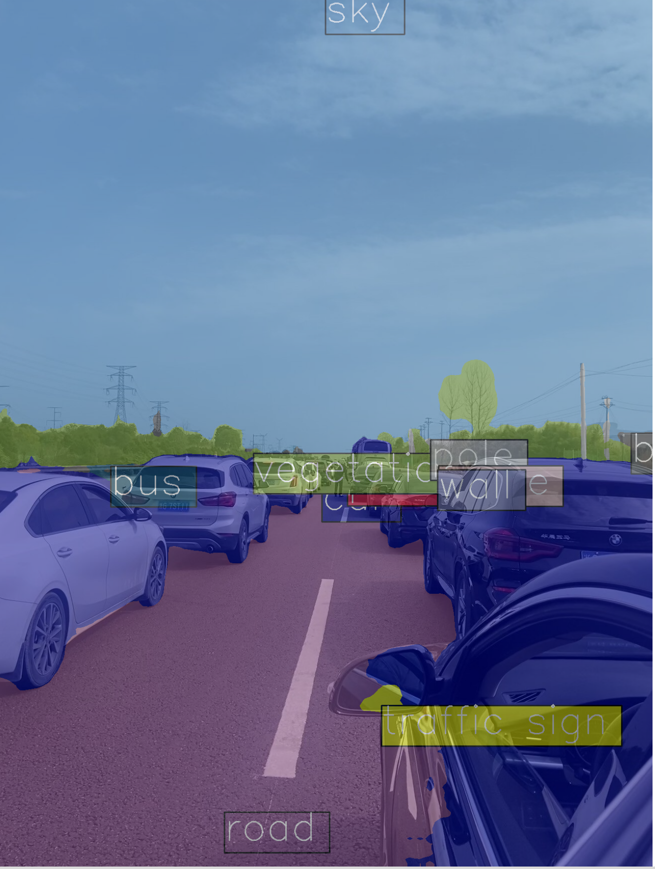
vis_result = show_result_pyplot(model, img_path, result, out_file='output_result.jpg', opacity=0.5) # opacity控制分割掩码的透明度
print("分割结果已保存至 'output_result.jpg'")测试结果

总结
通过CNN图像分类、YOLOv11目标检测和MMSegmentation语义分割三项工程实践,我们系统探索了视觉AI的核心任务和技术实现。这些实践表明,成功的视觉AI项目需要模型架构、数据质量和训练策略三者的协同优化。同时,视觉AI技术正从专用模型向通用大模型演进,面临多模态融合、效率优化、可信可靠等重要挑战。未来,随着物理启发模型、仿生设计等新思路的引入,视觉AI有望在更多实际场景中发挥更大价值,推动人工智能技术在产业中的深度融合与创新应用。

有“AI”的1024 = 2048,欢迎大家加入2048 AI社区
更多推荐


 27
27 0
0- 0


 已为社区贡献1条内容

所有评论(0)