小红书社区搜索算法二面

一、用了对比损失吧，手撕一下（项目中用了对比学习）

对比损失的核心思想是：

• 相似的样本对（label=1）距离应尽可能小
• 不相似的样本对（label=0）距离应超过 margin

数学公式：

给定两个样本的嵌入表示 x1, x2，标签 y ∈ {0,1}，margin为m，损失函数定义如下：
$$L=y\ast D^2+(1-y)\ast max(0,m-D{)}^2$$
其中：

• D = ||x1 - x2|| 表示两个样本的欧氏距离
• y = 1 表示正样本对
• y = 0 表示负样本对
• margin 是希望负样本之间的最小距离

import torch
import torch.nn.functional as F

def contrastive_loss(x1, x2, y, margin=1.0):
    # 欧氏距离
    dist = F.pairwise_distance(x1, x2)
    
    # 对比损失
    loss = y * dist.pow(2) + (1 - y) * torch.clamp(margin - dist, min=0.0).pow(2)
    
    return loss.mean()

```python
import torch
import torch.nn.functional as F

def contrastive_loss(x1, x2, label, margin=1.0):
    """
    计算对比损失 (Contrastive Loss)

    参数:
        x1, x2: shape = [batch_size, embedding_dim]，成对的样本嵌入向量
        label: shape = [batch_size]，1 表示正样本对，0 表示负样本对
        margin: 对于负样本对，拉开的最小距离

    返回:
        标量 loss
    """
    # 欧式距离
    distances = F.pairwise_distance(x1, x2, keepdim=True)  # shape: [batch_size, 1]

    # Contrastive Loss 公式
    loss_pos = label * torch.pow(distances, 2)             # 正样本对损失
    loss_neg = (1 - label) * torch.pow(torch.clamp(margin - distances, min=0.0), 2)  # 负样本对损失

    loss = 0.5 * (loss_pos + loss_neg)
    return loss.mean()

二、召回的工作做得挺多，召回能用什么损失函数？

2.1. 二分类损失（Binary Classification Loss）

损失函数	说明	适用场景
Binary Cross-Entropy	最常用，优化点击/转化概率	用户-物品是否点击/召回
Focal Loss	关注难分类样本，缓解类别不平衡	类别极度不平衡的召回任务

2.2. 排序损失（Ranking Loss）

损失函数	说明	优点	框架支持
Pairwise Ranking Loss（BPR）	正负样本对得分比较	符合推荐目标	PyTorch, TensorFlow
Triplet Loss	三元组(anchor, positive, negative)	简单有效的embedding学习	PyTorch内置支持
Contrastive Loss	强化正负样本embedding距离差异	多用于embedding召回	需自定义实现
Margin Ranking Loss	控制正负样本得分差 ≥ margin	通用且易优化	PyTorch内置支持
InfoNCE / NT-Xent Loss	对比学习损失，用于无监督/自监督	提升embedding质量	推荐+对比学习结合场景

2.2.1. BPR Loss（Bayesian Personalized Ranking）

BPR Loss 是推荐召回中非常经典的pairwise ranking loss，目的是让正样本得分比负样本得分高。
$${\mathcal{L}}_{\text{BPR}}=-\log (\sigma ({\hat{y}}_{ui}-{\hat{y}}_{uj}))$$

• ${\hat{y}}_{ui}$：用户 $u$ 对正样本物品 $i$ 的预测得分
• ${\hat{y}}_{uj}$：用户 $u$ 对负样本物品 $j$ 的预测得分
• $\sigma (\cdot )$：Sigmoid 函数

import torch

def bpr_loss(pos_scores, neg_scores):
    diff = pos_scores - neg_scores
    loss = -torch.mean(torch.log(torch.sigmoid(diff) + 1e-8))
    return loss

pos_scores = torch.tensor([3.0, 4.0, 5.0])
neg_scores = torch.tensor([1.0, 2.0, 1.0])
loss = bpr_loss(pos_scores, neg_scores)
print("BPR Loss:", loss.item())

2.2.2. Triplet Loss（三元组损失）

Triplet Loss 用于强化 anchor 和 positive 的距离比 anchor 和 negative 的距离更近，通常用于 embedding 学习。
$${\mathcal{L}}_{\text{Triplet}}=\max (0,d(a,p)-d(a,n)+\text{margin})$$

• $a$：anchor 向量（用户或查询）
• $p$：positive 向量（相关物品）
• $n$：negative 向量（无关物品）
• $d(\cdot ,\cdot )$：距离函数（如欧氏距离或余弦距离）
• $\text{margin}$：预定义的间隔常数，用于控制正负样本之间的最小差距

import torch
import torch.nn as nn
triplet_loss = nn.TripletMarginLoss(margin=1.0, p=2)
anchor = torch.randn(4, 128)
positive = torch.randn(4, 128)
negative = torch.randn(4, 128)
loss = triplet_loss(anchor, positive, negative)
print("Triplet Loss:", loss.item())

2.2.3. Margin Ranking Loss（边缘排序损失）

$${\mathcal{L}}_{\text{Ranking}}=\max (0,-y\cdot (x_1-x_2)+\text{margin})$$

• $x_1$、$x_2$：两个样本的得分
• $y$：标签，取值为 1 表示 $x_1$ 应大于 $x_2$，-1 表示相反
• $\text{margin}$：定义正负样本得分间的最小差距
• 当 $y=1$，模型应让 $x_1>x_2+\text{margin}$
• 当 $y=-1$，模型应让 $x_1<x_2-\text{margin}$

如果当前排序已经满足 margin 要求，损失为 0；否则会进行惩罚。

import torch
import torch.nn as nn
margin_ranking_loss = nn.MarginRankingLoss(margin=1.0)
pos_scores = torch.tensor([3.0, 4.0, 5.0])
neg_scores = torch.tensor([1.0, 2.0, 1.0])
y = torch.ones(pos_scores.size())  # 标签，1表示pos > neg

loss = margin_ranking_loss(pos_scores, neg_scores, y)
print("Margin Ranking Loss:", loss.item())

三、BatchNorm 的训练与推理差异及可训练参数

3.1. 训练阶段（Training）

• 使用 当前 mini-batch 的均值和方差 来进行标准化：
  $${\mu }_B=\frac{1}{m}\sum _{i=1}^m{x}_i,{\sigma }_B^2=\frac{1}{m}\sum _{i=1}^m(x_i-{\mu }_B{)}^2$$
• 对每个特征进行标准化：
  $${\hat{x}}_i=\frac{x_i-{\mu }_B}{\sqrt{{\sigma }_B^2+ϵ}}$$
• 使用可学习的缩放因子和偏移参数：
  $$y_i=\gamma {\hat{x}}_i+\beta$$
• 更新全局的移动平均均值和方差（用于推理阶段）：
  • moving_mean
  • moving_variance

3.2. 推理阶段（Inference / Evaluation）

• 使用训练过程中累积的 moving mean 和 moving variance：
  $${\hat{x}}_i=\frac{x_i-\text{moving\_mean}}{\sqrt{\text{moving\_variance}+ϵ}}$$
• 同样使用 γ 和 β 进行缩放和平移：
  $$y_i=\gamma {\hat{x}}_i+\beta$$
• 不再更新任何统计量。

3.3 可训练参数（Trainable Parameters）

BatchNorm 中的两个可训练参数是：

• gamma (γ)：缩放因子（scale）
• beta (β)：偏移因子（shift）
  这两个参数的作用是：
• 允许模型恢复原始的特征表达能力（如果需要）。
• 在归一化之后仍保持模型表达能力。

3.4. 非可训练参数（缓冲区参数）

这些参数在训练过程中更新，但不进行反向传播：

• running_mean（即 moving_mean）
• running_var（即 moving_variance）

model.train() # 设置为训练模式，使用batch统计量
model.eval() # 设置为推理模式，使用moving统计量

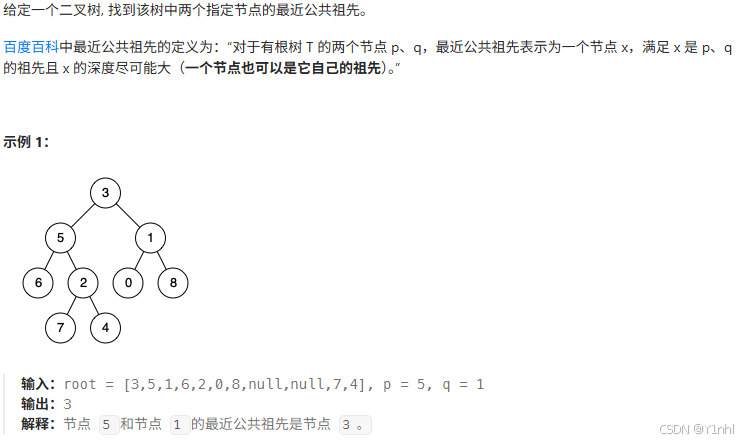
四、236. 二叉树的最近公共祖先

class Solution:
    def lowestCommonAncestor(self, root: 'TreeNode', p: 'TreeNode', q: 'TreeNode') -> 'TreeNode':
        if not root or root == p or root == q:
            return root
        left = self.lowestCommonAncestor(root.left, p, q)
        right = self.lowestCommonAncestor(root.right, p, q)
        if not left:
            return right
        if not right:
            return left
        return root       # 如果 left和right都有返回，返回这个root（公共节点）

五、4. 寻找两个正序数组的中位数

class Solution:
    def findMedianSortedArrays(self, a: List[int], b: List[int]) -> float:
        if len(a) > len(b):
            a, b = b, a  # 保证下面的 i 可以从 0 开始枚举

        m, n = len(a), len(b)
        a = [-inf] + a + [inf]
        b = [-inf] + b + [inf]

        # 枚举 nums1 有 i 个数在第一组
        # 那么 nums2 有 j = (m + n + 1) // 2 - i 个数在第一组
        i, j = 0, (m + n + 1) // 2
        while True:
            if a[i] <= b[j + 1] and a[i + 1] > b[j]:  # 写 >= 也可以
                max1 = max(a[i], b[j])  # 第一组的最大值
                min2 = min(a[i + 1], b[j + 1])  # 第二组的最小值
                return max1 if (m + n) % 2 else (max1 + min2) / 2
            i += 1  # 继续枚举
            j -= 1