矢量拟合(4)极点和残差形式的传递函数与等效电路
数学描述矢量拟合的思想是通过一组有理函数的模型来拟合一组频率响应的采样点(例如S,Y和Z矩阵)。模型定义为拉普拉斯传递函数。H‾(s‾)=d+s‾e+∑k=1Kc‾ks‾−p‾k\mathbf{\underline{H}}(\mathrm{\underline{s}}) = \mathbf{d} + \mathrm{\underline{s}} \mathbf{e} + \sum_{k=1}^K
数学描述
矢量拟合的思想是通过一组有理函数的模型来拟合一组频率响应的采样点(例如S,Y和Z矩阵)。
模型定义为拉普拉斯传递函数。
H‾(s‾)=d+s‾e+∑k=1Kc‾ks‾−p‾k \mathbf{\underline{H}}(\mathrm{\underline{s}}) = \mathbf{d} + \mathrm{\underline{s}} \mathbf{e} + \sum_{k=1}^K \frac{\underline{\mathbf{c}}_{k}}{\mathrm{\underline{s}} - \underline{p}_k} H(s)=d+se+k=1∑Ks−pkck
在每一个采样点ωn\omega_nωn,都应该有:
H‾(s‾=jωn)=!H‾sampled(ωn) \begin{equation} \mathbf{\underline{H}}(\mathrm{\underline{s}} = \mathrm{j} \omega_n) \overset{!}{=} \mathbf{\underline{H}}_\mathrm{sampled}(\omega_n) \end{equation} H(s=jωn)=!Hsampled(ωn)
H‾(s‾)\mathbf{\underline{H}}(\mathrm{\underline{s}})H(s)是一个向量(矢量),包括一组模型的复数响应H‾1(s‾)\underline{H}_1(\mathrm{\underline{s}})H1(s),H‾2(s‾)\underline{H}_2(\mathrm{\underline{s}})H2(s),… H‾M(s‾)\underline{H}_M(\mathrm{\underline{s}})HM(s)。
H‾(s‾)\mathbf{\underline{H}}(\mathrm{\underline{s}})H(s)中的所有的元素共享一组复数极点p‾k\underline{p}_kpk,但是却有独立的不同的复数残差c‾k\mathbf{\underline{c}}_kck和不同的实数常数d\mathbf{d}d以及实数的比例系数e\mathbf{e}e。
即:
p‾=(p‾1p‾2p‾3⋯p‾K) \begin{equation} \mathbf{\underline{p}} = \begin{pmatrix} \underline{p}_1 & \underline{p}_2 & \underline{p}_3 & \cdots & \underline{p}_K \end{pmatrix} \end{equation} p=(p1p2p3⋯pK)
c‾=(c‾1,1c‾2,1c‾3,1⋯c‾K,1c‾1,2c‾2,2c‾3,2⋯c‾K,2⋮c‾1,Mc‾2,Mc‾3,M⋯c‾K,M) \begin{equation} \mathbf{\underline{c}} = \begin{pmatrix} \underline{c}_{1,1} & \underline{c}_{2,1} & \underline{c}_{3,1} & \cdots & \underline{c}_{K,1} \\ \underline{c}_{1,2} & \underline{c}_{2,2} & \underline{c}_{3,2} & \cdots & \underline{c}_{K,2} \\ \vdots\\ \underline{c}_{1,M} & \underline{c}_{2,M} & \underline{c}_{3,M} & \cdots & \underline{c}_{K,M} \\ \end{pmatrix} \end{equation} c=
c1,1c1,2⋮c1,Mc2,1c2,2c2,Mc3,1c3,2c3,M⋯⋯⋯cK,1cK,2cK,M
d=(d1d2⋮dM) \begin{equation} \mathbf{d} = \begin{pmatrix} d_1 \\ d_2 \\ \vdots \\ d_M \end{pmatrix} \end{equation} d=
d1d2⋮dM
e=(e1e2⋮eM) \begin{equation} \mathbf{e} = \begin{pmatrix} e_1 \\ e_2 \\ \vdots \\ e_M \end{pmatrix} \end{equation} e=
e1e2⋮eM
要实现H‾(s‾)\mathbf{\underline{H}}(\mathrm{\underline{s}})H(s)很好地拟合到H‾sampled\mathbf{\underline{H}}_\mathrm{sampled}Hsampled
极点的数量K,取决于响应的形状。
- 极点 表示系统的动态特性,决定了系统对输入信号的响应方式。
- 响应的形状(例如急剧变化、振荡行为或平滑变化)决定了准确建模或逼近该行为所需的极点数量。
- 如果响应是平滑的,可能只需要少量极点即可获得良好的拟合。
- 如果响应具有急剧变化或包含多种振荡成分,则可能需要更多的极点以捕捉其复杂性。
二端口S参数的拟合
(S‾11(ω1)S‾12(ω1)S‾21(ω1)S‾22(ω1)⋮S‾11(ωN)S‾12(ωN)S‾21(ωN)S‾22(ωN))=!(d11+jω1e11+∑k=1Kc‾k,11jω1−p‾kd12+jω1e12+∑k=1Kc‾k,12jω1−p‾kd21+jω1e21+∑k=1Kc‾k,21jω1−p‾kd22+jω1e22+∑k=1Kc‾k,22jω1−p‾k⋮d11+jωNe11+∑k=1Kc‾k,11jωN−p‾kd12+jωNe12+∑k=1Kc‾k,12jωN−p‾kd21+jωNe21+∑k=1Kc‾k,21jωN−p‾kd22+jωNe22+∑k=1Kc‾k,22jωN−p‾k) \begin{equation} \begin{pmatrix} \underline{S}_{11}(\omega_1) \\ \underline{S}_{12}(\omega_1) \\ \underline{S}_{21}(\omega_1) \\ \underline{S}_{22}(\omega_1) \\ \vdots \\ \underline{S}_{11}(\omega_\mathrm{N}) \\ \underline{S}_{12}(\omega_\mathrm{N}) \\ \underline{S}_{21}(\omega_\mathrm{N}) \\ \underline{S}_{22}(\omega_\mathrm{N}) \end{pmatrix} \overset{!}{=} \begin{pmatrix} d_{11} + \mathrm{j} \omega_1 e_{11} + \sum_{k=1}^K \frac{\underline{c}_{k,11}}{\mathrm{j} \omega_1 - \underline{p}_k} \\ d_{12} + \mathrm{j} \omega_1 e_{12} + \sum_{k=1}^K \frac{\underline{c}_{k,12}}{\mathrm{j} \omega_1 - \underline{p}_k} \\ d_{21} + \mathrm{j} \omega_1 e_{21} + \sum_{k=1}^K \frac{\underline{c}_{k,21}}{\mathrm{j} \omega_1 - \underline{p}_k} \\ d_{22} + \mathrm{j} \omega_1 e_{22} + \sum_{k=1}^K \frac{\underline{c}_{k,22}}{\mathrm{j} \omega_1 - \underline{p}_k} \\ \vdots \\ d_{11} + \mathrm{j} \omega_\mathrm{N} e_{11} + \sum_{k=1}^K \frac{\underline{c}_{k,11}}{\mathrm{j} \omega_\mathrm{N} - \underline{p}_k} \\ d_{12} + \mathrm{j} \omega_\mathrm{N} e_{12} + \sum_{k=1}^K \frac{\underline{c}_{k,12}}{\mathrm{j} \omega_\mathrm{N} - \underline{p}_k} \\ d_{21} + \mathrm{j} \omega_\mathrm{N} e_{21} + \sum_{k=1}^K \frac{\underline{c}_{k,21}}{\mathrm{j} \omega_\mathrm{N} - \underline{p}_k} \\ d_{22} + \mathrm{j} \omega_\mathrm{N} e_{22} + \sum_{k=1}^K \frac{\underline{c}_{k,22}}{\mathrm{j} \omega_\mathrm{N} - \underline{p}_k} \end{pmatrix} \end{equation} S11(ω1)S12(ω1)S21(ω1)S22(ω1)⋮S11(ωN)S12(ωN)S21(ωN)S22(ωN) =! d11+jω1e11+∑k=1Kjω1−pkck,11d12+jω1e12+∑k=1Kjω1−pkck,12d21+jω1e21+∑k=1Kjω1−pkck,21d22+jω1e22+∑k=1Kjω1−pkck,22⋮d11+jωNe11+∑k=1KjωN−pkck,11d12+jωNe12+∑k=1KjωN−pkck,12d21+jωNe21+∑k=1KjωN−pkck,21d22+jωNe22+∑k=1KjωN−pkck,22
等效电路
常数和比例项
d+s‾e\mathbf{d} + \mathrm{\underline{s}} \mathbf{e}d+se在等效电路中代表着等效的阻Z‾RL(s‾)\underline{Z}_\mathrm{RL}(\mathrm{\underline{s}})ZRL(s)或等效导纳Y‾RC(s‾)\underline{Y}_\mathrm{RC}(\mathrm{\underline{s}})YRC(s)。
在等效电路中可以通过RL串联电路和RC并联电路实现。
常数和比例项的目标响应:
H‾target(s‾)=di+s‾ei \begin{equation} \underline{H}_\mathrm{target}(\mathrm{\underline{s}}) = d_i + \mathrm{\underline{s}} e_i \end{equation} Htarget(s)=di+sei
RL串联电路的阻抗为:
Z‾RL(s‾)=R+s‾L \begin{equation} \underline{Z}_\mathrm{RL}(\mathrm{\underline{s}}) = R + \mathrm{\underline{s}} L \end{equation} ZRL(s)=R+sL
其中R=diR = d_iR=di,L=eiL = e_iL=ei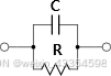
RC并联电路的导纳为:
Y‾RC(s‾)=1R+s‾C \begin{equation} \underline{Y}_\mathrm{RC}(\mathrm{\underline{s}}) = \frac{1}{R} + \mathrm{\underline{s}} C \end{equation} YRC(s)=R1+sC
其中R=1diR = \frac{1}{d_i}R=di1,C=eiC = e_iC=ei
通过将传递函数写成极点和残差的形式可以更加直观地反应出系统的动态特性,且易于实现数值的计算。
实数的极点和残差传递函数的形式如下:
H‾target(s‾)=ck,is‾−pk,i \begin{equation} \underline{H}_\mathrm{target}(\mathrm{\underline{s}}) = \frac{c_{k,i}}{\mathrm{\underline{s}} - p_{k,i}} \end{equation} Htarget(s)=s−pk,ick,i
因此将RC电路的导纳传递函数改为阻抗传递函数:
Z‾RC(s‾)=1Cs‾+1RC \begin{equation} \underline{Z}_\mathrm{RC}(\mathrm{\underline{s}}) = \frac{\frac{1}{C}}{\mathrm{\underline{s}} + \frac{1}{RC}} \end{equation} ZRC(s)=s+RC1C1
同样的将RL串联电路的阻抗传递函数改为导纳传递函数:
Y‾RL(s‾)=1Ls‾+RL \begin{equation} \underline{Y}_\mathrm{RL}(\mathrm{\underline{s}}) = \frac{\frac{1}{L}}{\mathrm{\underline{s}} + \frac{R}{L}} \end{equation} YRL(s)=s+LRL1
复数极点p‾k=pk′+jpk′′\underline{p}_k = p'_k + \mathrm{j} p''_kpk=pk′+jpk′′和复数残差c‾k=ck′+jck′′\underline{c}_k = c'_k + \mathrm{j} c''_kck=ck′+jck′′,总是以共轭对的方式存在。
此时,目标传递函数为:
H‾target(s‾)=c‾ks‾−p‾k+c‾k∗s‾−p‾k∗=(ck+ck∗)s‾−(ckpk∗+ck∗pk)s‾2−(pk+pk∗)s‾+pkpk∗ \begin{equation} \underline{H}_\mathrm{target}(\mathrm{\underline{s}}) = \frac{\underline{c}_k}{\mathrm{\underline{s}} - \underline{p}_k} + \frac{\underline{c}^*_k}{\mathrm{\underline{s}} - \underline{p}^*_k} = \frac{(c_k+c_k^*) \mathrm{\underline{s}} - (c_k p_k^* + c_k^* p_k)}{\mathrm{\underline{s}}^2 - (p_k+p_k^*) \mathrm{\underline{s}} + p_kp_k^*} \end{equation} Htarget(s)=s−pkck+s−pk∗ck∗=s2−(pk+pk∗)s+pkpk∗(ck+ck∗)s−(ckpk∗+ck∗pk)
这个传递函数可以用两种不同的等效电路来表示。
1. 串联和并联RCL电路加上额外的电流和电压源
串联RCL电路加上额外的电流源
串联RLC电路的导纳:
YˉRL(s)=Iˉ(s)Vˉ(s)=1(R+sL+1sC)=sLs2+sRL+1LC \begin{equation} \bar{Y}_{RL}(s)=\frac{\bar{I}(s)}{\bar{V}(s)}=\frac{1}{(R+sL+\frac{1}{sC})}=\frac{\frac{s}{L}}{s^2+s\frac{R}{L}+\frac{1}{LC}} \end{equation} YˉRL(s)=Vˉ(s)Iˉ(s)=(R+sL+sC1)1=s2+sLR+LC1Ls
极点pk,pk∗=−R2L±j1LC−(R2L)2 with(R2L)2<1LCp_k,p^*_k=-\frac{R}{2L}±j\sqrt{\frac{1}{LC}-(\frac{R}{2L})^2} \space \space with (\frac{R}{2L})^2<\frac{1}{LC}pk,pk∗=−2LR±jLC1−(2LR)2 with(2LR)2<LC1
残差ck=pkL2j1LC−(R2L)2c_k=\frac{\frac{p_k}{L}}{2j\sqrt{\frac{1}{LC}-(\frac{R}{2L})^2}}ck=2jLC1−(2LR)2Lpk, ck∗=−pk∗L2j1LC−(R2L)2c_k^*=-\frac{\frac{p_k^*}{L}}{2j\sqrt{\frac{1}{LC}-(\frac{R}{2L})^2}}ck∗=−2jLC1−(2LR)2Lpk∗
L=1ck+ck∗ \begin{equation} L=\frac{1}{c_k+c_k^*} \end{equation} L=ck+ck∗1
R=−pk+pk∗ck+ck∗ \begin{equation} R=-\frac{p_k+p_k^*}{c_k+c_k^*} \end{equation} R=−ck+ck∗pk+pk∗
C=ck+ck∗pkpk∗ \begin{equation} C=\frac{c_k+c_k^*}{p_kp_k^*} \end{equation} C=pkpk∗ck+ck∗
串联RLC的导纳传递函数式(14)只包含了共轭复数极点残差一般形式的传递函数中的前一项,缺少了后一项:
−(ckpk∗+ck∗pk)s‾2−(pk+pk∗)s‾+pkpk∗ \begin{equation} \frac{- (c_k p_k^* + c_k^* p_k)}{\mathrm{\underline{s}}^2 - (p_k+p_k^*) \mathrm{\underline{s}} + p_kp_k^*} \end{equation} s2−(pk+pk∗)s+pkpk∗−(ckpk∗+ck∗pk)
式(18)的分子为一个常数项,用bbb来表示。
即
b=−(ckpk∗+ck∗pk) \begin{equation} b=-(c_kp_k^*+c_k^*p_k) \end{equation} b=−(ckpk∗+ck∗pk)
共轭复数极点残差一般形式的传递函数中分子包含sss的前一项和后一项常数项的分母是相同的。
因此用一个额外项添加到RLC串联导纳传递函数的后面,构成了极点残差的一般形式为:
F(s)=YˉRLC(s)+Fadd(s)=sLs2+sRL+1LC+Fadd(s) \begin{equation} F(s)=\bar{Y}_{RLC}(s)+F_{add}(s)=\frac{\frac{s}{L}}{s^2+s\frac{R}{L}+\frac{1}{LC}}+F_{add}(s) \end{equation} F(s)=YˉRLC(s)+Fadd(s)=s2+sLR+LC1Ls+Fadd(s)
其中
Fadd=bs2+sRL+1LC \begin{equation} F_{add}=\frac{b}{s^2+s\frac{R}{L}+\frac{1}{LC}} \end{equation} Fadd=s2+sLR+LC1b
电容C的分压比为:
VC(s)VRLC(s)=1LC1s2+sRL+1LC \begin{equation} \frac{V_C(s)}{V_{RLC}(s)}=\frac{1}{LC}\frac{1}{s^2+s\frac{R}{L}+\frac{1}{LC}} \end{equation} VRLC(s)VC(s)=LC1s2+sLR+LC11
因此
Fadd(s)=bLCVC(s)VRLC(s) \begin{equation} F_{add}(s)=bLC\frac{V_C(s)}{V_{RLC}(s)} \end{equation} Fadd(s)=bLCVRLC(s)VC(s)
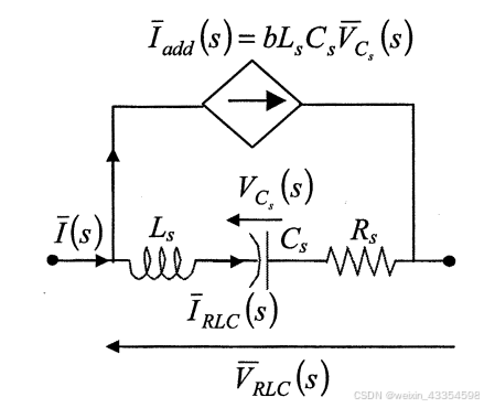
式(23)可以看作一个电流源的并联内导纳。
因此电流源总的电流为:
Iˉ(s)=IˉRLC+Iˉadd(s)=YˉRLC(s)VˉRLC(s)+bLCVˉC(s) \begin{equation} \bar{I}(s)=\bar{I}_{RLC}+\bar{I}_{add}(s)=\bar{Y}_{RLC}(s)\bar{V}_{RLC}(s)+bLC\bar{V}_{C}(s) \end{equation} Iˉ(s)=IˉRLC+Iˉadd(s)=YˉRLC(s)VˉRLC(s)+bLCVˉC(s)
从式(24)可以看出,这是一个压控电流源,通过电容的电压控制电流,bLCbLCbLC为比例系数。
并联RCL电路加上额外的电压源
同样的,也可以用并联的RLC电路的阻抗来表示共轭复数极点残差形式的传递函数。
极点为:
pk,pk∗=−12RC±j1LC−(12RC)2 with(12RC)2<1LC \begin{equation} p_k,p^*_k=-\frac{1}{2RC}±j\sqrt{\frac{1}{LC}-(\frac{1}{2RC})^2} \space \space with (\frac{1}{2RC})^2<\frac{1}{LC} \end{equation} pk,pk∗=−2RC1±jLC1−(2RC1)2 with(2RC1)2<LC1
残差为:
ck=pkC2j1LC−(12RC)2 \begin{equation} c_k=\frac{\frac{p_k}{C}}{2j\sqrt{\frac{1}{LC}-(\frac{1}{2RC})^2}} \end{equation} ck=2jLC1−(2RC1)2Cpk
ck∗=−pk∗C2j1LC−(12RC)2 \begin{equation} c_k^*=-\frac{\frac{p_k^*}{C}}{2j\sqrt{\frac{1}{LC}-(\frac{1}{2RC})^2}} \end{equation} ck∗=−2jLC1−(2RC1)2Cpk∗
传递函数F(s)F(s)F(s)为:
F(s)=ZˉRLC(s)+Fadd(s)=sCs2+s1RC+1LC+bs2+s1RC+1LC \begin{equation} F(s)=\bar{Z}_{RLC}(s)+F_{add}(s)=\frac{\frac{s}{C}}{s^2+s\frac{1}{RC}+\frac{1}{LC}}+\frac{b}{s^2+s\frac{1}{RC}+\frac{1}{LC}} \end{equation} F(s)=ZˉRLC(s)+Fadd(s)=s2+sRC1+LC1Cs+s2+sRC1+LC1b
电感L上的分容比为:
IˉL(s)IˉRLC=1LC1s2+s1RC+1LC \begin{equation} \frac{\bar{I}_L(s)}{\bar{I}_{RLC}}=\frac{1}{LC}\frac{1}{s^2+s\frac{1}{RC}+\frac{1}{LC}} \end{equation} IˉRLCIˉL(s)=LC1s2+sRC1+LC11
因此
Fadd(s)=bLCIˉL(s)IˉRLC \begin{equation} F_{add}(s)=bLC\frac{\bar{I}_L(s)}{\bar{I}_{RLC}} \end{equation} Fadd(s)=bLCIˉRLCIˉL(s)
Fadd(s)F_{add}(s)Fadd(s)可以看作一个电压源串联的内阻抗
总的电压为:
Vˉ(s)=ZˉRLC(s)IˉRLC+bLCIˉL(s) \begin{equation} \bar{V}(s)=\bar{Z}_{RLC}(s)\bar{I}_{RLC}+bLC\bar{I}_L(s) \end{equation} Vˉ(s)=ZˉRLC(s)IˉRLC+bLCIˉL(s)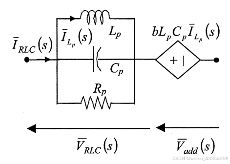
C=1ck+ck∗ \begin{equation} C=\frac{1}{c_k+c_k^*} \end{equation} C=ck+ck∗1
R=−ck+ck∗pk+pk∗ \begin{equation} R=-\frac{c_k+c_k^*}{p_k+p_k^*} \end{equation} R=−pk+pk∗ck+ck∗
L=ck+ck∗pkpk∗ \begin{equation} L=\frac{c_k+c_k^*}{p_kp_k^*} \end{equation} L=pkpk∗ck+ck∗
2. 串联LR与并联RC的组合电路
串联LR与并联RC的串联导纳
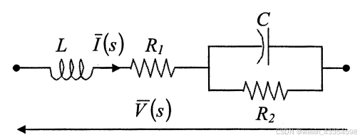
Y(s)=1Ls+1R2C(s2+(R1L+1R2C)s+(R1L1R2C+1LC)) \begin{equation} Y(s) = \frac{1}{L}\frac{s+\frac{1}{R_2C}}{ \left( s^2 + \left( \frac{R_1}{L} + \frac{1}{R_2 C} \right) s + \left( \frac{R_1}{L} \frac{1}{R_2 C} + \frac{1}{L C} \right) \right)} \end{equation} Y(s)=L1(s2+(LR1+R2C1)s+(LR1R2C1+LC1))s+R2C1
通过极点和残差可以确定等效电路中R1,R2,L,CR_1, R_2, L, CR1,R2,L,C的数值。
R1=1ck+ck∗[−(pk+pk∗)+1ck+ck∗(ckpk∗+ck∗pk)] \begin{equation} R_1=\frac{1}{c_k+c_k^*}[-(p_k+p_k^*)+\frac{1}{c_k+c_k^*}(c_kp_k^*+c_k^*p_k)] \end{equation} R1=ck+ck∗1[−(pk+pk∗)+ck+ck∗1(ckpk∗+ck∗pk)]
R2=−1C(ck+ck∗)ckpk∗+ck∗pk \begin{equation} R_2=-\frac{1}{C}\frac{(c_k+c_k^*)}{c_kp_k^*+c_k^*p_k} \end{equation} R2=−C1ckpk∗+ck∗pk(ck+ck∗)
L=1ck+ck∗ \begin{equation} L=\frac{1}{c_k+c_k^*} \end{equation} L=ck+ck∗1
C=ck+ck∗pkpk∗+[−(pk+pk∗)+1ck+ck∗(ckpk∗+ck∗pk)] \begin{equation} C=\frac{c_k+c_k^*}{p_kp_k^*+[-(p_k+p_k^*)+\frac{1}{c_k+c_k^*}(c_kp_k^*+c_k^*p_k)]} \end{equation} C=pkpk∗+[−(pk+pk∗)+ck+ck∗1(ckpk∗+ck∗pk)]ck+ck∗
串联LR与并联RC的并联阻抗
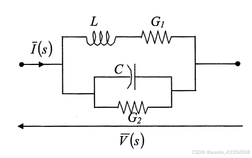
Z(s)=(s+1G1L)C(s2+(G2C+1G1L)s+(G2C1G1L+1LC)) \begin{equation} Z(s) = \frac{\left(s + \frac{1}{G_1 L}\right)}{C \left( s^2 + \left( \frac{G_2}{C} + \frac{1}{G_1 L} \right) s + \left( \frac{G_2}{C} \frac{1}{G_1 L} + \frac{1}{L C} \right) \right)} \end{equation} Z(s)=C(s2+(CG2+G1L1)s+(CG2G1L1+LC1))(s+G1L1)
通过极点和残差可以确定等效电路中G1,G2,L,CG_1, G_2, L, CG1,G2,L,C的数值。
G1=−1L1(ckpk∗+ck∗pk) \begin{equation} G_1 = -\frac{1}{L}\frac{1}{(c_kp_k^*+ c_k^*p_{k})} \end{equation} G1=−L1(ckpk∗+ck∗pk)1
G2=1ck+ck∗×[−(pk+pk∗)+1ck+ck∗(ckpk∗+ck∗pk)] \begin{equation} G_2 = \frac{1}{c_k + c_k^*} \times \left[ -(p_k + p_k^*) + \frac{1}{c_k + c_k^*}(c_k p_k^* + c_k^*p_k ) \right] \end{equation} G2=ck+ck∗1×[−(pk+pk∗)+ck+ck∗1(ckpk∗+ck∗pk)]
C=1ck+ck∗ \begin{equation} C = \frac{1}{c_k + c_k^*} \end{equation} C=ck+ck∗1
L=ck+ck∗pkpk∗+[−(pk+pk∗)+1ck+ck∗(ckpk∗+ck∗pk)×1ckpk∗+ck∗pkck+ck∗ \begin{equation} L = \frac{c_k+c_k^*}{p_kp_k^*+[-(p_k+p_k^*)+\frac{1}{c_k+c_k^*}(c_kp_k^*+c_k^*p_k)}\times\frac{1}{\frac{c_kp_k^*+c_k^*p_k}{c_k+c_k^*}} \end{equation} L=pkpk∗+[−(pk+pk∗)+ck+ck∗1(ckpk∗+ck∗pk)ck+ck∗×ck+ck∗ckpk∗+ck∗pk1

有“AI”的1024 = 2048,欢迎大家加入2048 AI社区
更多推荐


 5
5 0
0- 0


 已为社区贡献1条内容

所有评论(0)