sarima模型_如何通过sarima模型为时间序列建模_python

sarima模型

In this tutorial I will show you how to model a seasonal time series through a SARIMA model.

在本教程中，我将向您展示如何通过SARIMA模型对季节时间序列进行建模。

Here you can download the Jupyter notebook of the code described in this tutorial.

在这里，您可以下载本教程中描述的代码的Jupyter笔记本。

入门 (Getting Started)

将数据集转换为时间序列 (Convert the dataset into a time series)

In this example we will use the number of tourist arrivals to Italy. Data are extracted from the European Statistics: Annual Data on Tourism Industries. Firstly, we import the dataset related to foreign tourists arrivals in Italy from 2012 to 2019 October and then we convert it into a time series.

在此示例中，我们将使用前往意大利的游客人数。数据摘自《欧洲统计：旅游业年度数据》。首先，我们导入与2012年至2019年10月在意大利入境的外国游客有关的数据集，然后将其转换为时间序列。

In order to perform the conversion to time series, two steps are needed:

为了执行到时间序列的转换，需要两个步骤：

the column containing dates must be converted to datetime. This can be done through the function to_datetime(), which converts a string into a datetime.

包含日期的列必须转换为datetime。这可以通过函数to_datetime()完成，该函数将字符串转换为日期时间。
set the index of the dataframe to the column containing dates. This can be done through the function set_index() applied to the dataframe.

将数据框的索引设置为包含日期的列。这可以通过将函数set_index()应用于数据set_index()来完成。

import pandas as pddf = pd.read_csv('../sources/IT_tourists_arrivals.csv')
df['date'] = pd.to_datetime(df['date'])
df = df[df['date'] > '2012-01-01']
df.set_index('date', inplace=True)

We can get some useful statistics related to the time series through the describe() function.

我们可以通过describe()函数获得一些与时间序列有关的有用统计信息。

df.describe()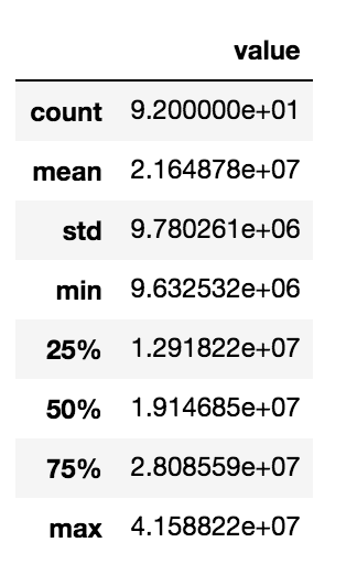

初步分析 (Preliminary analysis)

绘制时间序列以检查季节性 (Plot the time series to check the seasonality)

The preliminary analysis involves a visual analysis of the time series, in order to understand its general trend and behaviour. Firstly, we create the time series and we store it in the variable ts.

初步分析包括对时间序列的可视化分析，以便了解其总体趋势和行为。首先，我们创建时间序列并将其存储在变量ts 。

ts = df['value']

Then, we plot the ts trend. We use the matplotlib library provided by Python.

然后，我们绘制ts趋势。我们使用Python提供的matplotlib库。

import matplotlib.pylab as plt
plt.plot(ts)
plt.ylabel('Total Number of Tourists Arrivals')
plt.grid()
plt.tight_layout()
plt.savefig('plots/IT_tourists_arrivals.png')
plt.show()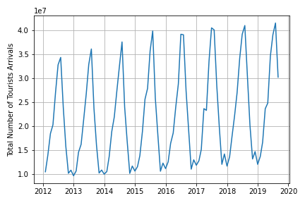

计算模型的参数 (Calculate the parameters for the model)

调整模型 (Tune the model)

We build a SARIMA model to represent the time series. SARIMA is an acronym for Seasonal AutoRegressive Integrated Moving Average. It is composed of two models AR and MA. The model is defined by three parameters:

我们建立了一个SARIMA模型来表示时间序列。 SARIMA是“季节性自回归综合移动平均线”的首字母缩写。它由两个模型AR和MA组成。该模型由三个参数定义：

d = degree of first differencing involved
d =涉及的一次微分的程度
p = order of the AR part
p = AR部分的顺序
q = order of the moving average part.
q =移动平均线部分的阶数。

The value of p can be determined through the ACF plot, which shows the autocorrelations which measure the relationship between an observation and its previous one. The value of d is the order of integration and can be calculated as the number of transformations needed to make the time series stationary. The value of q can be determined through the PACF plot.

可以通过ACF图确定p的值，该图显示了测量一个观测值与其前一个观测值之间的关系的自相关。 d的值是积分的阶数，可以计算为使时间序列平稳所需的变换次数。 q的值可以通过PACF图确定。

In order determine the value of d, we can perform the Dickey-Fuller test, which is able to verify whether a time series is stationary or not. We can use the adfuller class, contained in the statsmodels library. We define a function, called test_stationarity(), which returns True, if the time series is positive, False otherwise.

为了确定d的值，我们可以执行Dickey-Fuller测试，该测试可以验证时间序列是否稳定。我们可以使用statsmodels库中包含的adfuller类。我们定义了一个名为test_stationarity()的函数，如果时间序列为正，则返回True，否则返回False。

from statsmodels.tsa.stattools import adfullerdef test_stationarity(timeseries):
    dftest = adfuller(timeseries, autolag='AIC')
    dfoutput = pd.Series(dftest[0:4], index=['Test Statistic','p-value','#Lags Used','Number of Observations Used'])
    for key,value in dftest[4].items():
        dfoutput['Critical Value (%s)'%key] = value
    critical_value = dftest[4]['5%']
    test_statistic = dftest[0]
    alpha = 1e-3
    pvalue = dftest[1]
    if pvalue < alpha and test_statistic < critical_value:  # null hypothesis: x is non stationary
        print("X is stationary")
        return True
    else:
        print("X is not stationary")
        return False

We transform the time series through the diff() function as many times as the time series becomes stationary.

当时间序列变得平稳时，我们通过diff()函数对时间序列进行了多次转换。

ts_diff = pd.Series(ts)
d = 0
while test_stationarity(ts_diff) is False:
    ts_diff = ts_diff.diff().dropna()
    d = d + 1

In order to calculate the value of p and q, we can plot the ACF and PACF graphs, respectively. We can use the plot_acf() and plot_pacf() functions available in the statsmodels library. The value of p corresponds to the maximum value in the ACF graph external to the confidence intervals (shown in light blue). In our case, che correct value of p = 9.

为了计算p和q的值，我们可以分别绘制ACF和PACF图。我们可以使用statsmodels库中可用的plot_acf()和plot_pacf()函数。 p的值对应于置信区间外部的ACF图中的最大值(以浅蓝色显示)。在我们的情况下，p = 9的正确值。

from statsmodels.graphics.tsaplots import plot_acf, plot_pacf
plot_acf(ts_trend, lags =12)
plt.savefig('plots/acf.png')
plt.show()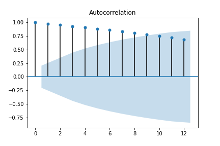

Similarly, the value of q corresponds to the maximum value in the PACF graph external to the confidence intervals (shown in light blue). In our case, che correct value of q = 1.

类似地，q的值对应于置信区间之外的PACF图中的最大值(以浅蓝色显示)。在我们的情况下，q等于1的正确值。

plot_pacf(ts_trend, lags =12)
plt.savefig('plots/pacf.png')
plt.show()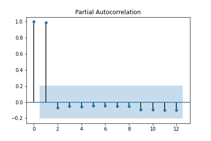

建立SARIMA模型 (Build the SARIMA model)

如何训练SARIMA模型 (How to train the SARIMA model)

Now we are ready to build the SARIMA model. We can use the SARIMAX class provided by the statsmodels library. We fit the model and get the prediction through the get_prediction() function. We can retrieve also the confidence intervals through the conf_int() function.

现在，我们准备构建SARIMA模型。我们可以使用statsmodels库提供的SARIMAX类。我们拟合模型并通过get_prediction()函数获得预测。我们还可以通过conf_int()函数检索置信区间。

from statsmodels.tsa.statespace.sarimax import SARIMAXp = 9
q = 1
model = SARIMAX(ts, order=(p,d,q))
model_fit = model.fit(disp=1,solver='powell')
fcast = model_fit.get_prediction(start=1, end=len(ts))
ts_p = fcast.predicted_mean
ts_ci = fcast.conf_int()

We plot results.

我们绘制结果。

plt.plot(ts_p,label='prediction')
plt.plot(ts,color='red',label='actual')
plt.fill_between(ts_ci.index[1:],
                ts_ci.iloc[1:, 0],
                ts_ci.iloc[1:, 1], color='k', alpha=.2)plt.ylabel('Total Number of Tourists Arrivals')
plt.legend()
plt.tight_layout()
plt.grid()
plt.savefig('plots/IT_trend_prediction.png')
plt.show()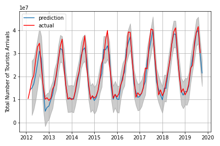

计算一些统计 (Calculate some statistics)

检查模型的性能 (Check the performance of the model)

Finally, we can calculate some statistics to evaluate the performance of the model. We calculate the Pearson’s coefficient, through the pearsonr() function provided by the scipy library.

最后，我们可以计算一些统计信息以评估模型的性能。我们通过scipy库提供的pearsonr()函数来计算Pearson系数。

from scipy import stats
stats.pearsonr(ts_trend_p[1:], ts[1:])

We also calculate the R squared metrics.

我们还计算R平方指标。

residuals = ts - ts_trend_p
ss_res = np.sum(residuals**2)
ss_tot = np.sum((ts-np.mean(ts))**2)
r_squared = 1 - (ss_res / ss_tot)
r_squared

学过的知识 (Lesson learned)

In this tutorial I have illustrated how to model a time series through a SARIMA model. Summarising, you should follow the following steps:

在本教程中，我说明了如何通过SARIMA模型对时间序列进行建模。总结一下，您应该遵循以下步骤：

convert your data frame into a time series
将您的数据帧转换为时间序列
calculate the values of p, d and q to tune the SARIMA model
计算p，d和q的值以调整SARIMA模型
build the SARIMA model with the calculated p, d and q values
使用计算的p，d和q值构建SARIMA模型
test the performance of the model.
测试模型的性能。

An improvement of the proposed model could involve the splitting of the time series in two parts: training and test sets. Usually, the training set is used to fit the model while the test set is used to calculate the performance of the model.

所提出模型的改进可能涉及将时间序列分为两部分：训练和测试集。通常，训练集用于拟合模型，而测试集用于计算模型的性能。