机器学习部分课后题(王衡军版)
机器学习(王衡军版)部分课后习题5.试编写程序,利用本章提供的k-means算法代码或者 sklearn.cluster. KMeans算法函数实现二分k-means算法,对随书资源中的kmeansSamples. txt文件中的点进行分簇,并与k-means算法的效果进行比较。
运行环境
按课本中讲解,采用Anaconda自带的Spyder和Jupyter Notebook 作为开发环境。
Anaconda下载安装
可到Anaconda 官方网站下载安装包安装。


完成之后,在Anaconda程序组里选择点击“Anaconda Navigator”,启动Navigator图形化管理界面
接下来打开Spyder即可
第二章部分课后题
![]()
# -*- coding: utf-8 -*-


import numpy as np

# Define the points
point1 = np.array([1, 2, 3])
point2 = np.array([3, 4, 8])

# Calculate L1 distance (Manhattan)
L1_distance = np.sum(np.abs(point1 - point2))

# Calculate L2 distance (Euclidean)
L2_distance = np.sqrt(np.sum((point1 - point2)**2))

# Calculate L∞ distance (Chebyshev)
L_inf_distance = np.max(np.abs(point1 - point2))

L1_distance, L2_distance, L_inf_distance
随书资源文件:
链接: https://pan.baidu.com/s/1L-iC95ByxayvxGFSKWPUsg?pwd=w8ws 提取码: w8ws
import numpy as np
import matplotlib.pyplot as plt

def L2(vecXi, vecXj):
    '''
    计算欧氏距离
    para vecXi:点坐标,向量
    para vecXj:点坐标,向量
    retrurn: 两点之间的欧氏距离
    '''
    return np.sqrt(np.sum(np.power(vecXi - vecXj, 2)))

def kMeans(S, k, distMeas=L2):
    '''
    K均值聚类
    para S:样本集,多维数组
    para k:簇个数
    para distMeas:距离度量函数,默认为欧氏距离计算函数
    return sampleTag:一维数组,存储样本对应的簇标记
    return clusterCents:一维数组,各簇中心
    retrun SSE:误差平方和
    '''
    m = np.shape(S)[0] # 样本总数
    sampleTag = np.zeros(m)

    # 随机产生k个初始簇中心
    n = np.shape(S)[1] # 样本向量的特征数
    clusterCents = np.mat([[-1.93964824,2.33260803],[7.79822795,6.72621783],[10.64183154,0.20088133]])
    #clusterCents = np.mat(np.zeros((k,n)))
    #for j in range(n):
    #    minJ = min(S[:,j])
    #    rangeJ = float(max(S[:,j]) - minJ)
    #    clusterCents[:,j] = np.mat(minJ + rangeJ * np.random.rand(k,1))

    sampleTagChanged = True
    SSE = 0.0
    while sampleTagChanged: # 如果没有点发生分配结果改变,则结束
        sampleTagChanged = False
        SSE = 0.0

        # 计算每个样本点到各簇中心的距离
        for i in range(m):
            minD = np.inf
            minIndex = -1
            for j in range(k):
                d = distMeas(clusterCents[j,:],S[i,:])
                if d < minD:
                    minD = d
                    minIndex = j
            if sampleTag[i] != minIndex:
                sampleTagChanged = True
            sampleTag[i] = minIndex
            SSE += minD**2
        print(clusterCents)
        plt.scatter(clusterCents[:,0].tolist(),clusterCents[:,1].tolist(),c='r',marker='^',linewidths=7)
        plt.scatter(S[:,0],S[:,1],c=sampleTag,linewidths=np.power(sampleTag+0.5, 2))
        plt.show()
        print(SSE)

        # 重新计算簇中心
        for i in range(k):
            ClustI = S[np.nonzero(sampleTag[:]==i)[0]]
            clusterCents[i,:] = np.mean(ClustI, axis=0)
    return clusterCents, sampleTag, SSE

if __name__=='__main__':
    samples = np.loadtxt("G:\spyder\kmeansSamples.txt")
    clusterCents, sampleTag, SSE = kMeans(samples, 3)
    #plt.scatter(clusterCents[:,0].tolist(),clusterCents[:,1].tolist(),c='r',marker='^')
    #plt.scatter(samples[:,0],samples[:,1],c=sampleTag,linewidths=np.power(sampleTag+0.5, 2))
    plt.show()
    print(clusterCents)
    print(SSE)
随书资源(p13页k-means代码):
链接: https://pan.baidu.com/s/1r-LcgG-sKLWRJ3KYgutOJQ?pwd=wtqd 提取码: wtqd
import numpy as np
import matplotlib.pyplot as plt

def L1(vecXi, vecXj):
    '''
    计算曼哈顿距离
    para vecXi:点坐标,向量
    para vecXj:点坐标,向量
    return: 两点之间的曼哈顿距离
    '''
    return np.sum(np.abs(vecXi - vecXj))

def kMedian(S, k, distMeas=L1):
    '''
    K-median 聚类
    para S:样本集,多维数组
    para k:簇个数
    para distMeas:距离度量函数,默认为曼哈顿距离计算函数
    return sampleTag:一维数组,存储样本对应的簇标记
    return clusterCents:一维数组,各簇中心
    retrun SSE:误差平方和
    '''
    m = np.shape(S)[0] # 样本总数
    sampleTag = np.zeros(m)

    # 随机产生k个初始簇中心
    n = np.shape(S)[1] # 样本向量的特征数
    clusterCents = np.mat([[-1.93964824,2.33260803],[7.79822795,6.72621783],[10.64183154,0.20088133]])

    sampleTagChanged = True
    SSE = 0.0
    while sampleTagChanged: # 如果没有点发生分配结果改变,则结束
        sampleTagChanged = False
        SSE = 0.0

        # 计算每个样本点到各簇中心的距离
        for i in range(m):
            minD = np.inf
            minIndex = -1
            for j in range(k):
                d = distMeas(clusterCents[j,:],S[i,:])
                if d < minD:
                    minD = d
                    minIndex = j
            if sampleTag[i] != minIndex:
                sampleTagChanged = True
            sampleTag[i] = minIndex
            SSE += minD

        plt.scatter(clusterCents[:,0].tolist(),clusterCents[:,1].tolist(),c='r',marker='^',linewidths=7)
        plt.scatter(S[:,0],S[:,1],c=sampleTag,linewidths=np.power(sampleTag+0.5, 2))
        plt.show()
        print(SSE)

        # 重新计算簇中心(中位数)
        for i in range(k):
            ClustI = S[np.nonzero(sampleTag[:]==i)[0]]  # 获取属于第i簇的所有点
            if len(ClustI) > 0:
                clusterCents[i,:] = np.median(ClustI, axis=0)  # 计算中位数
    return clusterCents, sampleTag, SSE

if __name__=='__main__':
    samples = np.loadtxt("G:\spyder\kmeansSamples.txt")
    clusterCents, sampleTag, SSE = kMedian(samples, 3)
    plt.show()
    print(clusterCents)
    print(SSE)
第三章部分课后题

import numpy as np
import matplotlib.pyplot as plt
from sklearn.linear_model import LinearRegression

# 数据
temperature = np.array([15, 20, 25, 30, 35, 40]).reshape(-1, 1)
flower_count = np.array([136, 140, 155, 160, 157, 175])

# 创建线性回归模型
model = LinearRegression()
model.fit(temperature, flower_count)

# 预测
predictions = model.predict(temperature)

# 输出结果
print("截距:", model.intercept_)
print("斜率:", model.coef_[0])

# 设置字体
plt.rcParams['font.sans-serif'] = ['SimHei']  # 使用黑体
plt.rcParams['axes.unicode_minus'] = False  # 使负号正常显示

# 可视化
plt.scatter(temperature, flower_count, color='blue', label='实际数据')
plt.plot(temperature, predictions, color='red', label='回归线')
plt.xlabel('温度')
plt.ylabel('花数量')
plt.title('温度与花数量的线性回归')
plt.legend()
plt.show()

随书资源(p55页代码3-6):
链接: https://pan.baidu.com/s/1-Kj-aiGxr7PJumPaxzPhQA?pwd=kc6s 提取码: kc6s
import numpy as np

def gradient(x, y, w):
    m, n = np.shape(x)
    g = np.mat(np.zeros((n, 1)))
    for i in range(m):
        err = y[i, 0] - x[i, :] * w
        for j in range(n):
            g[j, 0] -= err * x[i, j]
    return g

def lossValue(x, y, w):
    k = y - x * w
    return (k.T * k) / 2

temperatures = [15, 20, 25, 30, 35, 40]
flowers = [136, 140, 155, 160, 157, 175]
X = (np.mat([[1] * len(temperatures), temperatures])).T
y = (np.mat(flowers)).T

W = (np.mat([0.0, 0.0])).T
alpha = 0.01  # 初始学习率
decay_rate = 0.99  # 衰减率
loss_change = 0.000001
loss = lossValue(X, y, W)

for i in range(30000):
    W = W - alpha * gradient(X, y, W)
    newloss = lossValue(X, y, W)
    print(f"{i}: W0: {W[0, 0]}, W1: {W[1, 0]}, Loss: {newloss[0, 0]}")

    # 动态调整学习率
    alpha *= decay_rate

    if abs(loss - newloss) < loss_change:
        break
    loss = newloss

批梯度下降:
import numpy as np
import time

def gradient(x, y, w):
    m, n = np.shape(x)
    errors = y - x * w
    g = - (1/m) * (x.T * errors)
    return g

def lossValue(x, y, w):
    errors = y - x * w
    return (errors.T * errors) / (2 * len(y))

temperatures = [15, 20, 25, 30, 35, 40]
flowers = [136, 140, 155, 160, 157, 175]
X = (np.mat([[1] * len(temperatures), temperatures])).T
y = (np.mat(flowers)).T

# 批梯度下降
W_batch = (np.mat([0.0, 0.0])).T
alpha = 0.00025
loss_change = 0.000001
loss = lossValue(X, y, W_batch)

start_time = time.time()
for i in range(30000):
    W_batch = W_batch - alpha * gradient(X, y, W_batch)
    newloss = lossValue(X, y, W_batch)
    if abs(loss - newloss) < loss_change:
        break
    loss = newloss
end_time = time.time()

print("批梯度下降结果: W0:", W_batch[0, 0], "W1:", W_batch[1, 0])
print("批梯度下降时间:", end_time - start_time)
随机梯度下降:
import numpy as np
import time

def gradient(x, y, w):
    '''计算一阶导函数的值'''
    errors = y - x * w
    return - (x.T * errors) / len(y)

def lossValue(x, y, w):
    '''计算损失函数'''
    errors = y - x * w
    return (errors.T * errors) / (2 * len(y))

# 数据准备
temperatures = [15, 20, 25, 30, 35, 40]
flowers = [136, 140, 155, 160, 157, 175]
X = np.mat([[1] * len(temperatures), temperatures]).T  # 增加偏置项
y = np.mat(flowers).T

# 随机梯度下降
W_sgd = (np.random.rand(2, 1) * 0.01)  # 小随机初始化
alpha = 0.001  # 降低学习率
loss_change = 0.000001  # 收敛条件
loss_sgd = lossValue(X, y, W_sgd)

start_time = time.time()  # 开始计时
for i in range(30000):
    for j in range(len(y)):
        rand_index = np.random.randint(len(y))  # 随机选择一个样本
        x_i = X[rand_index, :]
        y_i = y[rand_index, :]
        W_sgd = W_sgd - alpha * gradient(x_i, y_i, W_sgd)  # 更新权重

    newloss = lossValue(X, y, W_sgd)  # 计算新的损失
    if np.isnan(newloss) or np.isnan(W_sgd).any():  # 检查 NaN
        print("出现 NaN,停止训练。")
        break
    if abs(loss_sgd - newloss) < loss_change:  # 收敛条件
        break
    loss_sgd = newloss
end_time = time.time()  # 结束计时

# 输出结果
print("随机梯度下降结果: W0:", W_sgd[0, 0], "W1:", W_sgd[1, 0])
print("随机梯度下降时间:", end_time - start_time)
第四章部分课后题

import math

def sum_of_each_label(samples):
    '''
    统计样本集中每一类标签label出现的次数
    para samples:list,样本的列表,每样本也是一个列表,样本的最后一项为label
    return sum_of_each_label:dictionary,各类样本的数量
    '''
    labels = [sample[-1] for sample in samples]
    sum_of_each_label = dict([(i,labels.count(i)) for i in labels])
    return sum_of_each_label

def info_entropy(samples):
    '''
    计算样本集的信息熵
    para samples:list,样本的列表,每样本也是一个列表,样本的最后一项为label
    return infoEntropy:float,样本集的信息熵
    '''
    # 统计每类标签的数量
    label_counts = sum_of_each_label(samples)

    # 计算信息熵 infoEntropy = -∑(p * log(p))
    infoEntropy = 0.0
    sumOfSamples = len(samples)
    for label in label_counts:
        p = float(label_counts[label])/sumOfSamples
        infoEntropy -= p * math.log(p,2)
    return infoEntropy

def split_samples(samples, f, fvalue):
    '''
    切分样本集
    para samples:list,样本的列表,每样本也是一个列表,样本的最后一项为label,其它项为特征
    para f: int,切分的特征,用样本中的特征次序表示
    para fvalue: float or int,切分特征的决策值
    output lsamples: list, 切分后的左子集
    output rsamples: list, 切分后的右子集
    '''
    lsamples = []
    rsamples = []
    for s in samples:
        if s[f] < fvalue:
            lsamples.append(s)
        else:
            rsamples.append(s)
    return lsamples, rsamples

def info_gain(samples, f, fvalue):
    '''
    计算切分后的信息增益
    para samples:list,样本的列表,每样本也是一个列表,样本的最后一项为label,其它项为特征
    para f: int,切分的特征,用样本中的特征次序表示
    para fvalue: float or int,切分特征的决策值
    output : float, 切分后的信息增益
    '''
    lson, rson = split_samples(samples, f, fvalue)
    return info_entropy(samples) - (info_entropy(lson)*len(lson) + info_entropy(rson)*len(rson))/len(samples)

def gini_index(samples):
    '''
    计算样本集的Gini指数
    para samples:list,样本的列表,每样本也是一个列表,样本的最后一项为label,其它项为特征
    output: float, 样本集的Gini指数
    '''
    sumOfSamples = len(samples)
    if sumOfSamples == 0:
        return 0
    label_counts = sum_of_each_label(samples)

    gini = 0
    for label in label_counts:
        gini = gini + pow(label_counts[label], 2)

    return 1 - float(gini) / pow(sumOfSamples, 2)

def gini_index_splited(samples, f, fvalue):
    '''
    计算切分后的基尼指数
    para samples:list,样本的列表,每样本也是一个列表,样本的最后一项为label,其它项为特征
    para f: int,切分的特征,用样本中的特征次序表示
    para fvalue: float or int,切分特征的决策值
    output : float, 切分后的基尼指数
    '''
    lson, rson = split_samples(samples, f, fvalue)
    return (gini_index(lson)*len(lson) + gini_index(rson)*len(rson))/len(samples)

if __name__ == "__main__":

    # 表3-1 某人相亲数据,依次为年龄、身高、学历、月薪特征和是否相亲标签
    blind_date = [[35, 176, 0, 20000, 0],
                  [28, 178, 1, 10000, 1],
                  [26, 172, 0, 25000, 0],
                  [29, 173, 2, 20000, 1],
                  [28, 174, 0, 15000, 1]]

    # 计算集合的信息熵
    print("样本集的信息熵:", info_entropy(blind_date))
    # OUTPUT:0.9709505944546686

    # 计算集合的信息增益
    print("按身高175切分的信息增益:", info_gain(blind_date, 1, 175)) # 按身高175切分
    # OUTPUT:0.01997309402197478
    print("按学历是否硕士切分的信息增益:", info_gain(blind_date, 2, 1)) # 按学历是否硕士切分
    # OUTPUT:0.4199730940219748
    print("按月薪10000切分的信息增益:", info_gain(blind_date, 3, 10000)) # 按月薪10000切分
    # OUTPUT:0.0

    # 计算集合的基尼指数
    print("样本集的基尼指数:", gini_index(blind_date))
    # OUTPUT:0.48

    # 计算切分后的基尼指数
    print("按身高175切分后的基尼指数:", gini_index_splited(blind_date, 1, 175)) # 按身高175切分
    # OUTPUT:0.4666666666666667
    print("按学历是否硕士切分后的基尼指数:", gini_index_splited(blind_date, 2, 1)) # 按学历是否硕士切分
    # OUTPUT:0.26666666666666666
    print("按月薪10000切分后的基尼指数:", gini_index_splited(blind_date, 3, 10000)) # 按月薪10000切分
    # OUTPUT:0.48

    # 计算按年龄>=29切分的信息增益和基尼指数
    age_threshold = 29
    print(f"按年龄>= {age_threshold} 切分后信息增益:", info_gain(blind_date, 0, age_threshold))
    # OUTPUT: 0.17095059445466854
    print(f"按年龄>= {age_threshold} 切分后的基尼指数:", gini_index_splited(blind_date, 0, age_threshold))
    # OUTPUT: 0.3
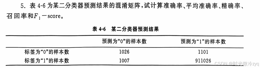
from sklearn.metrics import accuracy_score, precision_score, recall_score, f1_score, confusion_matrix

# 混淆矩阵的数值
conf_matrix = [[1026, 1101],
               [1007, 911026]]

# 将混淆矩阵转为对应的标签和预测结果
y_true = [0]*1026 + [0]*1101 + [1]*1007 + [1]*911026
y_pred = [0]*1026 + [1]*1101 + [0]*1007 + [1]*911026

# 计算准确率
accuracy = accuracy_score(y_true, y_pred)
print(f"准确率 (Accuracy): {accuracy}")

# 计算精确率
precision = precision_score(y_true, y_pred)
print(f"精确率 (Precision): {precision}")

# 计算召回率
recall = recall_score(y_true, y_pred)
print(f"召回率 (Recall): {recall}")

# 计算 F1-score
f1 = f1_score(y_true, y_pred)
print(f"F1-score: {f1}")

# 打印混淆矩阵
print("混淆矩阵:")
print(confusion_matrix(y_true, y_pred))

随书资源:通过网盘分享的文件:ellipseSamples.txt
链接: https://pan.baidu.com/s/11llthdDiejhK23rrYsaIMQ?pwd=5zvm 提取码: 5zvm
--来自百度网盘超级会员v5的分享
import numpy as np
import pandas as pd
import matplotlib.pyplot as plt
from sklearn.linear_model import LogisticRegression
from sklearn.model_selection import train_test_split
from sklearn.preprocessing import StandardScaler

# 加载数据,并使用正确的路径处理
data = pd.read_csv(r"G:\spyder\ellipseSamples.txt", delim_whitespace=True, header=None)
print(data.head())  # 查看数据是否正确加载

# 提取特征和标签
X = data.iloc[:, :-1].values  # 特征
y = data.iloc[:, -1].values   # 标签

# 标准化特征
scaler = StandardScaler()
X = scaler.fit_transform(X)

# 拆分训练集和测试集
X_train, X_test, y_train, y_test = train_test_split(X, y, test_size=0.2, random_state=42)

# 训练逻辑回归模型
model = LogisticRegression()
model.fit(X_train, y_train)

# 画出决策边界
def plot_decision_boundary(X, y, model):
    x_min, x_max = X[:, 0].min() - 1, X[:, 0].max() + 1
    y_min, y_max = X[:, 1].min() - 1, X[:, 1].max() + 1
    xx, yy = np.meshgrid(np.arange(x_min, x_max, 0.01),
                         np.arange(y_min, y_max, 0.01))

    Z = model.predict(np.c_[xx.ravel(), yy.ravel()])
    Z = Z.reshape(xx.shape)

    plt.contourf(xx, yy, Z, alpha=0.8)
    plt.scatter(X[:, 0], X[:, 1], c=y, edgecolors='k', marker='o', s=100)
    plt.xlabel('Feature 1')
    plt.ylabel('Feature 2')
    plt.title('Decision Boundary of Logistic Regression')
    plt.show()

# 绘制决策边界
plot_decision_boundary(X, y, model)

随书资源(优惠券使用实例资源):通过网盘分享的文件:tianchio2o
链接: https://pan.baidu.com/s/1AeJYGzOFtJVaXQUdJjJpOw?pwd=czhx 提取码: czhx
--来自百度网盘超级会员v5的分享
第五章部分课后题
![]()
随书资源:通过网盘分享的文件:tianchio2o
链接: https://pan.baidu.com/s/1AeJYGzOFtJVaXQUdJjJpOw?pwd=czhx 提取码: czhx
--来自百度网盘超级会员v5的分享
部分代码:
# 转换 Date_received 和 Date 为 datetime 格式
df['Date_received'] = pd.to_datetime(df['Date_received'], format='%Y%m%d', errors='coerce')
df['Date'] = pd.to_datetime(df['Date'], format='%Y%m%d', errors='coerce')
# 生成交叉表,显示领取日和核销日的分布
crosstab = pd.crosstab(df_used['received_dayofweek'], df_used['used_dayofweek'])
# 将数据转换为马赛克图可用的字典格式
mosaic_data = {(f'Received {int(row)}', f'Used {int(col)}'): crosstab.loc[row, col]
               for row in crosstab.index for col in crosstab.columns}
# 绘制马赛克图
plt.figure(figsize=(12, 8))
mosaic(mosaic_data, title='Coupon Redemption by Day of the Week')
plt.show()
奇异值:
随书资源(p142实例):通过网盘分享的文件:奇异值分解降维.ipynb
链接: https://pan.baidu.com/s/1o0YIxKnlaJi_Uk6SoFxoPA?pwd=sg99 提取码: sg99
--来自百度网盘超级会员v5的分享
import numpy as np
import matplotlib.pyplot as plt
from sklearn.decomposition import PCA

# 原始数据矩阵
A = np.array([[1, 2, 3, 4],
              [5, 6, 7, 8],
              [9, 10, 11, 12]])

print("原始矩阵 A:")
print(A)

# 使用 SVD 进行降维
U, sigma, VT = np.linalg.svd(A)
print("U:", U)
print("sigma:", sigma)
print("VT:", VT)

# 选择前1个主成分
sigma_c = np.diag(sigma[0:1])
U_c = U[:, 0:1]
VT_c = VT[0:1, :]
print("降维后的矩阵 U_c:", U_c)
print("降维后的矩阵 sigma_c:", sigma_c)
print("降维后的矩阵 VT_c:", VT_c)

# 重构矩阵
A_reconstructed_svd = U_c @ sigma_c @ VT_c
print("通过 SVD 降维重构的矩阵:")
print(A_reconstructed_svd)

# 使用 PCA 进行降维
pca = PCA(n_components=1)  # 选择一个主成分
A_reduced = pca.fit_transform(A)  # 这里将 A 作为 ndarray 传入

print("通过 PCA 降维得到的矩阵:")
print(A_reduced)

# 进行重构
A_reconstructed_pca = pca.inverse_transform(A_reduced)
print("通过 PCA 降维重构的矩阵:")
print(A_reconstructed_pca)

# 可视化降维效果(如果有需要)
plt.scatter(A[:, 0], A[:, 1], color='blue', label='Original Data', alpha=0.5)
plt.scatter(A_reduced[:, 0], np.zeros_like(A_reduced[:, 0]), color='red', label='PCA Reduced Data', alpha=0.5)
plt.title('PCA Dimensionality Reduction')
plt.xlabel('First Principal Component')
plt.ylabel('Zero (since we reduced to 1D)')
plt.legend()
plt.show()
主成分分析:
随书资源(p146实例):通过网盘分享的文件:主成分分析示例.ipynb
链接: https://pan.baidu.com/s/1cK5hMrDMgqt68ABELaqRyw?pwd=9si1 提取码: 9si1
--来自百度网盘超级会员v5的分享
import numpy as np
import matplotlib.pyplot as plt
from sklearn.decomposition import PCA

# 原始数据矩阵
X = np.array([[4, 2],
              [0, 2],
              [-2, 0],
              [-2, -4]])

print("原始矩阵 X:")
print(X)

# 使用 numpy 计算协方差矩阵
cov_matrix = np.cov(X.T)  # 转置以便计算列的协方差
print("协方差矩阵:")
print(cov_matrix)

# 计算特征值和特征向量
tr, W = np.linalg.eig(cov_matrix)
print("特征值:")
print(tr)
print("特征向量:")
print(W)

# 使用 sklearn 的 PCA 进行降维
pca = PCA(n_components=1)  # 选择一个主成分
X_reduced = pca.fit_transform(X)

print("通过 PCA 降维得到的矩阵:")
print(X_reduced)

# 进行重构
X_reconstructed = pca.inverse_transform(X_reduced)
print("通过 PCA 降维重构的矩阵:")
print(X_reconstructed)

# 绘制原始数据点和降维后的数据点
plt.scatter(X[:, 0], X[:, 1], color='blue', label='Original Data', alpha=0.5)
plt.scatter(X_reduced, np.zeros_like(X_reduced), color='red', label='PCA Reduced Data', alpha=0.5)
plt.title('PCA Dimensionality Reduction')
plt.xlabel('First Principal Component')
plt.ylabel('Zero (since we reduced to 1D)')
plt.legend()
plt.show()
第六章部分课后题
![]()
随书资源(代码6-4):通过网盘分享的文件:隐马尔可夫模型.ipynb
链接: https://pan.baidu.com/s/1eZ66rxEiXlr8RjZ4alYYtw?pwd=cfwi 提取码: cfwi
--来自百度网盘超级会员v5的分享
import numpy as np

# 状态空间I
states = {0, 1, 2}
# 初始状态概率向量π
pi = np.array([0.25, 0.5, 0.25])
# 状态转移矩阵A
A = np.array([[0,   1, 0],
              [0.5, 0, 0.5],
              [0,   1, 0]])

# 观测集合V
observations = {2, 3, 4, 5, 6, 7, 8, 9, 10, 11, 12}
# 观测概率矩阵B
B = np.array([[1/36, 2/36, 3/36, 4/36, 5/36, 6/36, 5/36, 4/36, 3/36, 2/36, 1/36],
              [1/24, 2/24, 3/24, 4/24, 4/24, 4/24, 3/24, 2/24, 1/24, 0,    0   ],
              [1/16, 2/16, 3/16, 4/16, 3/16, 2/16, 1/16, 0,    0,    0,    0   ]])

# 前向算法
def forward(pi, A, B, observ_list):
    N = A.shape[0]  # 状态总数
    T = len(observ_list)  # 列表长度
    table = np.zeros((N, T))  # 前向算法计算表
    table[:, 0] = pi * B[:, observ_list[0] - 2]  # 初始值

    for t in range(1, T):
        for i in range(N):
            table[i, t] = np.dot(table[:, t-1], A[:, i]) * B[i, observ_list[t] - 2]

    return table

# 计算观测序列 [10, 11, 7] 的概率
observ_list = [10, 11, 7]
table = forward(pi, A, B, observ_list)

# 计算观测序列的总概率
probability = np.sum(table[:, -1])
print("观测序列 [10, 11, 7] 的概率:", probability)

import numpy as np

# 状态空间I
states = {0, 1, 2}
# 初始状态概率向量π
pi = np.array([0.25, 0.5, 0.25])
# 状态转移矩阵A
A = np.array([[0,   1, 0],
              [0.5, 0, 0.5],
              [0,   1, 0]])

# 观测集合V
observations = {2, 3, 4, 5, 6, 7, 8, 9, 10, 11, 12}
# 观测概率矩阵B
B = np.array([[1/36, 2/36, 3/36, 4/36, 5/36, 6/36, 5/36, 4/36, 3/36, 2/36, 1/36],
              [1/24, 2/24, 3/24, 4/24, 4/24, 4/24, 3/24, 2/24, 1/24, 0,    0   ],
              [1/16, 2/16, 3/16, 4/16, 3/16, 2/16, 1/16, 0,    0,    0,    0   ]])

# 维特比算法
def viterbi(pi, A, B, observ_list):
    N = A.shape[0]  # 状态数
    T = len(observ_list)  # 观测序列长度
    viterbi_table = np.zeros((N, T))  # Viterbi 表
    backpointer = np.zeros((N, T), dtype=int)  # 回溯指针

    # 初始化
    viterbi_table[:, 0] = pi * B[:, observ_list[0] - 2]

    # 递推
    for t in range(1, T):
        for j in range(N):
            max_prob = -1
            for i in range(N):
                prob = viterbi_table[i, t-1] * A[i, j] * B[j, observ_list[t] - 2]
                if prob > max_prob:
                    max_prob = prob
                    backpointer[j, t] = i
            viterbi_table[j, t] = max_prob

    # 找到最大概率的最终状态
    best_path_prob = np.max(viterbi_table[:, -1])
    best_last_state = np.argmax(viterbi_table[:, -1])

    # 回溯
    best_path = [best_last_state]
    for t in range(T-1, 0, -1):
        best_last_state = backpointer[best_last_state, t]
        best_path.insert(0, best_last_state)

    return best_path, best_path_prob

# 计算观测序列 [10, 11, 7] 的最大可能状态序列
observ_list = [10, 11, 7]
best_path, best_path_prob = viterbi(pi, A, B, observ_list)

# 输出结果
print("观测序列 [10, 11, 7] 的最大可能状态序列:", best_path)
print("最大概率:", best_path_prob)
第七章部分课后题

随书资源:通过网盘分享的文件:7.4.1作业.ipynb
链接: https://pan.baidu.com/s/1qGTYIbD-VJfs_x-iNA85Tw?pwd=c8sk 提取码: c8sk
--来自百度网盘超级会员v5的分享
随书资源(课本p198):通过网盘分享的文件:误差反向传播算法示例.ipynb
链接: https://pan.baidu.com/s/10QsmJ320NFzYjVyIDaVIvA?pwd=u4ip 提取码: u4ip
--来自百度网盘超级会员v5的分享
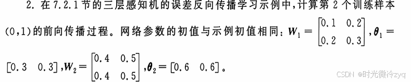
import numpy as np

# 样本实例
XX = np.array([[0.0,0.0],
              [0.0,1.0],
              [1.0,0.0],
              [1.0,1.0]])
# 样本标签
L = np.array([[0.0,1.0],
              [1.0,0.0],
              [1.0,0.0],
              [0.0,1.0]])
a = 0.5 # 步长
W1 = np.array([[0.1, 0.2], # 第1隐层的连接权重系数
               [0.2, 0.3]])
theta1 = np.array([0.3, 0.3]) # 第1隐层的阈值
W2 = np.array([[0.4, 0.5],  # 第2隐层的连接权重系数
               [0.4, 0.5]])
theta2 = np.array([0.6, 0.6]) # 第2隐层的阈值

Y1 = np.zeros(2) # 第1隐层的输出
Y2 = np.zeros(2) # 第2隐层的输出

def sigmoid(x):
    return 1/(1+np.exp(-x))

# 计算第1隐层节点1的输出
def y_1_1(W1, theta1, X):
    return sigmoid(W1[0,0]*X[0] + W1[1,0]*X[1] + theta1[0])

# 计算第1隐层节点2的输出
def y_1_2(W1, theta1, X):
    return sigmoid(W1[0,1]*X[0] + W1[1,1]*X[1] + theta1[1])

# 计算第2隐层节点1的输出
def y_2_1(W2, theta2, Y1):
    return sigmoid(W2[0,0]*Y1[0] + W2[1,0]*Y1[1] + theta2[0])

# 计算第2隐层节点2的输出
def y_2_2(W2, theta2, Y1):
    return sigmoid(W2[0,1]*Y1[0] + W2[1,1]*Y1[1] + theta2[1])

# 选择第2个训练样本 (0, 1)
X = XX[1]

# 前向传播过程
# 计算第1隐层的输出
Y1[0] = y_1_1(W1, theta1, X)
Y1[1] = y_1_2(W1, theta1, X)

# 计算第2隐层的输出
Y2[0] = y_2_1(W2, theta2, Y1)
Y2[1] = y_2_2(W2, theta2, Y1)

# 输出结果
print("第1隐层的输出 Y1: ", Y1)
print("第2隐层的输出 Y2: ", Y2)
![]()
import numpy as np
import tensorflow as tf
import matplotlib.pyplot as plt
import time

# 目标函数
def myfun(x):
    '''目标函数'''
    return 10 + 5 * x + 4 * x**2 + 6 * x**3

# 数据准备
x = np.array([-3.        , -2.68421053, -2.36842105, -2.05263158, -1.73684211, -1.42105263,
              -1.10526316, -0.78947368, -0.47368421, -0.15789474,  0.15789474,  0.47368421,
               0.78947368,  1.10526316,  1.42105263,  1.73684211,  2.05263158,  2.36842105,
               2.68421053,  3.        ])  # 转换为 NumPy 数组
y = np.array([-83.60437309, -109.02680368,  -99.45599857,  -72.85246379,   24.27643468,
               22.32819066,   13.0134867 ,  -37.47252415,  -16.24274272,   21.5705342 ,
              -12.63210639,   35.16554616,   42.58380499,   21.97718399,   19.50677405,
              107.2591151,   67.41705564,   95.78691168,  130.32069909,  253.31473912])  # 转换为 NumPy 数组
yy = y.copy()

# 数据标准化
miny = min(y)
maxy = max(y)

def standard(y, miny, maxy):
    step = maxy - miny
    return (y - miny) / step

def invstandard(y, miny, maxy):
    step = maxy - miny
    return miny + y * step

y_normalized = standard(y, miny, maxy)

# 自定义余弦相似度损失函数
def cosine_similarity(y_true, y_pred):
    return 1 - tf.reduce_sum(y_true * y_pred) / (tf.norm(y_true) * tf.norm(y_pred))

# 双曲余弦对数损失函数
def hyperbolic_cosine_log_loss(y_true, y_pred):
    return tf.reduce_mean(tf.log(1 + tf.square(y_pred - y_true)))

# 定义模型
def create_model(loss_function):
    model = tf.keras.Sequential([
        tf.keras.Input(shape=(1,)),  # 使用 Input 层
        tf.keras.layers.Dense(10, activation='sigmoid',
                              kernel_initializer='random_uniform', bias_initializer='zeros'),
        tf.keras.layers.Dense(1, activation='linear',
                              kernel_initializer='random_uniform', bias_initializer='zeros')
    ])
    model.compile(optimizer='sgd', loss=loss_function)
    return model

# 训练并可视化结果
def train_and_plot(loss_function, epochs):
    model = create_model(loss_function)

    # 训练时间记录
    start_time = time.time()
    model.fit(x.reshape(-1, 1), y_normalized, batch_size=10, epochs=epochs, verbose=0)
    training_time = time.time() - start_time

    # 可视化结果
    plt.figure(figsize=(10, 6))
    plt.title(f"损失函数: {loss_function} | 训练时间: {training_time:.2f} 秒")
    plt.scatter(x, yy, color="black", linewidth=2, label='原始数据')

    x1 = np.linspace(-3, 3, 100).reshape(-1, 1)
    y0 = myfun(x1)
    plt.plot(x1, y0, color="red", linewidth=1, label='真实函数')

    y1 = model.predict(x1)
    y1 = invstandard(y1, miny, maxy)
    plt.plot(x1, y1, "b--", linewidth=1, label='模型预测')

    plt.legend()
    plt.grid(True)
    plt.show()

# 定义不同的损失函数
loss_functions = [
    ('binary_crossentropy', '交叉熵'),
    ('mean_squared_error', '均方误差'),
    ('mean_absolute_error', '平均绝对误差'),  # 新增一个损失函数进行比较
    (cosine_similarity, '余弦相似度'),            # 使用自定义的余弦相似度损失函数
    (hyperbolic_cosine_log_loss, '双曲余弦对数')  # 使用自定义的双曲余弦对数损失函数
]

# 训练并可视化每个损失函数的效果
for loss_function, display_name in loss_functions:
    train_and_plot(loss_function, epochs=500)

随书资源:通过网盘分享的文件:误差反向传播算法示例.ipynb等2个文件
链接: https://pan.baidu.com/s/14QUWcmWFFrJHcdDR1Tkdfw?pwd=b55n 提取码: b55n
--来自百度网盘超级会员v5的分享
部分代码:
# 定义不同结构的模型
def create_model(layers):
    model = tf.keras.Sequential()
    # 输入层 + 隐层
    for units in layers:
        model.add(tf.keras.layers.Dense(units, activation='sigmoid',
                                        kernel_initializer='random_uniform', bias_initializer='zeros'))
    # 输出层
    model.add(tf.keras.layers.Dense(1, activation='sigmoid',
                                    kernel_initializer='random_uniform', bias_initializer='zeros'))
    # 编译模型
    model.compile(optimizer='sgd', loss='mean_squared_error')
    return model
图7-11:
# 不同模型的层数配置
layer_configs = {
    '三层 (1,1,1)': [1, 1],
    '三层 (1,2,1)': [1, 2],
    '四层 (1,5,5,1)': [1, 5, 5],
    '五层 (1,10,15,10,1)': [1, 10, 15, 10]
}
# 训练并显示结果
def train_and_plot(model_name, layers):
model = create_model(layers)
# 减少 epochs,增加日志输出
model.fit(x, y, batch_size=10, epochs=1000, verbose=1)
# 可视化结果
plt.figure()
plt.title(f"{model_name} 拟合结果")
plt.scatter(x, yy, color="black", linewidth=2, label='原始数据')
x1 = np.linspace(-3, 3, 100).reshape(-1, 1)
y0 = myfun(x1)
plt.plot(x1, y0, color="red", linewidth=1, label='真实函数')
y1 = model.predict(x1)
invstandard(y1, miny, maxy)
plt.plot(x1, y1, "b--", linewidth=1, label='模型预测')
plt.legend()
plt.show()图7-12:
# 训练并显示结果
def train_and_plot(epochs):
    model = create_model()
    model.fit(x, y, batch_size=10, epochs=epochs, verbose=0)

    # 可视化结果
    plt.figure()
    plt.title(f"{epochs} 轮训练结果")
    plt.scatter(x, yy, color="black", linewidth=2, label='原始数据')

    x1 = np.linspace(-3, 3, 100).reshape(-1, 1)
    y0 = myfun(x1)
    plt.plot(x1, y0, color="red", linewidth=1, label='真实函数')

    y1 = model.predict(x1)
    invstandard(y1, miny, maxy)
    plt.plot(x1, y1, "b--", linewidth=1, label='模型预测')

    plt.legend()
    plt.show()
# 训练并可视化不同轮数的模型
epochs_list = [1000, 3000, 5000, 10000]
for epochs in epochs_list:
train_and_plot(epochs)图7-13:
  # 训练模型
    model.fit(x, y_data, batch_size=10, epochs=3000, verbose=0)

    # 可视化结果
    plt.figure()
    plt.title(title)
    plt.scatter(x, yy, color="black", linewidth=2, label='原始数据')

    x1 = np.linspace(-3, 3, 100).reshape(-1, 1)
    y0 = myfun(x1)
    plt.plot(x1, y0, color="red", linewidth=1, label='真实函数')

    y1 = model.predict(x1)

    # 如果是归一化数据,进行反归一化
    if title == "归一化处理拟合结果":
        y1 = invstandard(y1, miny, maxy)

    plt.plot(x1, y1, "b--", linewidth=1, label='模型预测')

    plt.legend()
    plt.show()

# 分别生成归一化和不归一化处理的拟合结果
train_and_plot(y_normalized, "归一化处理拟合结果")
train_and_plot(y, "不归一化处理拟合结果")

# 定义模型
def create_model(loss_function):
    model = tf.keras.Sequential([
        tf.keras.Input(shape=(1,)),  # 使用 Input 层
        tf.keras.layers.Dense(10, activation='sigmoid',
                              kernel_initializer='random_uniform', bias_initializer='zeros'),
        tf.keras.layers.Dense(1, activation='linear',
                              kernel_initializer='random_uniform', bias_initializer='zeros')
    ])
    model.compile(optimizer='sgd', loss=loss_function)
    return model
# 训练时间记录
start_time = time.time()
model.fit(x.reshape(-1, 1), y_normalized, batch_size=10, epochs=epochs, verbose=0)
training_time = time.time() - start_time# 定义不同的损失函数
loss_functions = [
('binary_crossentropy', '交叉熵'),
('mean_squared_error', '均方误差'),
('mean_absolute_error', '平均绝对误差'), # 新增一个损失函数进行比较
(cosine_similarity, '余弦相似度'), # 使用自定义的余弦相似度损失函数
(hyperbolic_cosine_log_loss, '双曲余弦对数') # 使用自定义的双曲余弦对数损失函数
]本文内容仅用于学习参考,请勿用于其他用途。如有问题,可评论区交流

有“AI”的1024 = 2048,欢迎大家加入2048 AI社区
更多推荐


 32
32 0
0- 0


 已为社区贡献2条内容

所有评论(0)