单变量线性回归

#----------- 导入必要的包 -------------#
import numpy as np
import pandas as pd
import matplotlib.pyplot as plt

#----------- 读取数据 -------------#
PATH = 'ex1data1.txt'

data = pd.read_csv(PATH, header=None, names=['Population', 'Profit'])
print(data.head())

# 新增一列，x0(截距项）
data.insert(0, 'Ones', 1)
print(data.head())

# 将输入的x和输出的y分开
# 列数
cols = data.shape[1]
X = data.iloc[:, 0:cols-1]
Y = data.iloc[:,cols-1:cols]

# pandas中的DataFrame类型的数据转换为numpy矩阵
X = np.matrix(X.values)
Y = np.matrix(Y.values)
# theta初始化为0
Theta = np.matrix(np.array([[0], [0]]))
print(Theta)


# 代价函数
def cost_function(x, y, theta):
    # theta.T表示矩阵的转置
    inner = np.power(x*theta - y, 2)
    return np.sum(inner) / (2*len(x))


# 接着进行梯度下降的计算
# 这个是batch梯度下降，数据量比较小，采用这种方式的消耗可控
# 所设置的参数有学习率，参数theta， 矩阵Y和矩阵X
def gradient_descent(alpha, theta, x, y):
    theta = theta + x.T * (alpha * (y-x*theta)) / x.shape[0]
    return theta


# 开始进行梯度下降，设置初始学习率为0.001。可以通过设置轮数来作为梯度下降的条件。
# 也可以采取判断两次参数之间的差距作为判断，当两个参数之间的差距很小的时候，就可以认为达到了收敛
# 同时记录每一次的损失函数，之后画出一个损失随着轮数的变化
old_Theta = Theta
Alpha = 0.01
cost_list = []
iters = 1000
condition = np.matrix(np.array([[0.0001], [0.0001]]))
while True:
    cost = cost_function(X, Y, old_Theta)
    cost_list.append(cost)
    Theta = gradient_descent(alpha=Alpha, theta=old_Theta, x=X, y=Y)
    if (np.abs(Theta - old_Theta) < condition).all():
        break
    old_Theta = Theta

print(len(cost_list))

# 画出损失函数的图像
h_axis = np.linspace(1, len(cost_list),num=len(cost_list))
print(h_axis)
plt.plot(h_axis,cost_list)
plt.show()

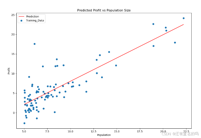
# 绘制出自己拟合的直线的图像
x1 = np.linspace(data.Population.min(), data.Population.max(), 100)
y1 = Theta[0, 0] + Theta[1, 0] * x1
plt.figure(figsize=(12, 8))
plt.xlabel("Population")
plt.ylabel("Profit")
l1 = plt.plot(x1, y1, label="Prediction", color='red')
l2 = plt.scatter(data.Population, data.Profit, label="Training_Data")
plt.legend(loc='best')
plt.title('Predicted Profit vs Population Size')
plt.show()

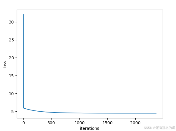
单变量线性回归损失曲线：

所拟合的曲线图

多变量线性回归

#------------- 导包 ------------------#
import numpy as np
import pandas
import matplotlib.pyplot as plt
# 这里需要导入一个三维的库，以展示数据的分布
from mpl_toolkits.mplot3d import Axes3D

# 文件路径
PATH = 'ex1data2.txt'
data = pandas.read_csv(PATH, header=None, names=["Area", 'Numbers of bedroom', 'Profit'])
print(data.describe())

# 记录Area, Numbers_of_bedroom, Profit的一些特征，用于后面进行参数转换
means = data.mean().values 
# 这样数据就从Pandas的DataFrame类型转换成了numpy数据类型
stds = data.std().values
mins = data.min().values
maxs = data.max().values

data1 = data  # 用一个新的变量记录原数据，方便画出原数据的散点图
# 由于房屋面积和房间个数这两个特征的取值范围差距太大，需要进行特征缩放。
# 将特征进行正规化缩放，如果不进行特征缩放，计算量会超过计算机内存
data = (data - data.mean()) / data.std()    
# mean()方法计算平均值，std()方法计算标准差

print(data.head())
# 将输入特征和标签分隔开来
columns = data.shape[1]
X = data.iloc[:, 0:columns-1]
Y = data.iloc[:, columns-1:]

# 在X中新增一列
# x0本身没有参与正规化
X.insert(0, 'ones', 1)
print(X.head())

# 将 DataFrame 的值转换为 numpy矩阵
new_x = np.matrix(X.values)
new_y = np.matrix(Y.values)

# theta的初始值
theta = np.matrix(np.array([[0], [0], [0]]))


# 设置损失函数(和单变量完全相同）
def cost_function(theta_1, x_1, y_1):
    inner = np.power((x_1*theta_1) - y_1, 2)
    return np.sum(inner) / (2 * len(x_1))

# 设置梯度下降(和单变量完全相同)
def gradient_descent(theta_1, alpha, x_1, y_1):
    theta_1 = theta_1 - alpha / len(x_1) * x_1.T * (x_1 * theta_1 - y_1)
    return theta_1

# 设置学习率，训练轮数和损失列表
alpha = 0.005 
iters = 3000
cost_list = []

# 进行梯度下降 
#（这里没有将进行的梯度下降过程直接写在函数里，写在了函数里的话会更加方便）
for i in range(iters):
    cost = cost_function(theta, new_x, new_y)
    cost_list.append(cost)
    theta = gradient_descent(theta, alpha, new_x, new_y)

# 绘制损失函数曲线图
iters_list = np.linspace(1, len(cost_list), len(cost_list))
plt.plot(iters_list, cost_list)
plt.xlabel('iters')
plt.ylabel('loss')
plt.show()

means = means.reshape(-1,1)  # 本来的形状是（3，）转换为（3，1）
stds = means.reshape(-1,1)
theta = np.array(theta)  # 将numpy类型的矩阵转为为数组，一般不要使用矩阵这个类

# 参数转化为原来的参数
def theta_transform(theta, means, stds):
    temp = means[:-1] * theta[1:] / stds[:-1]
    theta[0] = (theta[0] - np.sum(temp)) * stds[-1] + means[-1]
    theta[1:] = theta[1:] * stds[-1] / stds[:-1]
    return theta  # -1表示不指定列数
theta = theta_transform(theta,means,stds)

#可以用一个例子进行一下预测
def predictPrice(x, y, theta):
    return theta[0, 0] + theta[1, 0]*x + theta[1, 0]*y
print(predictPrice(2104,3,theta))

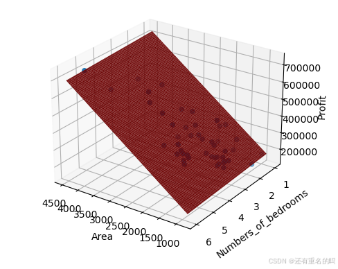
# #绘制拟合平面
fig = plt.figure()
ax = fig.add_subplot(111, projection='3d')
ax.view_init(elev=25, azim=125)

ax.set_xlabel('Area')
ax.set_ylabel('Numbers_of_bedrooms')
ax.set_zlabel('Profit')
ax.scatter(data1.iloc[:,0], data1.iloc[:,1], data1.iloc[:,2])
X_ = np.linspace(data1.iloc[:, 0].min(), data1.iloc[:, 0].max()+1, 100)
Y_ = np.linspace(data1.iloc[:, 1].min(), data1.iloc[:, 1].max()+1, 100)
X_, Y_ = np.meshgrid(X_, Y_)
Z_ = theta[0,0] + theta[1,0] * X_ + theta[2,0] * Y_
ax.plot_surface(X_, Y_, Z_, rstride=1, cstride=1, color='red')
plt.show()

所拟合出的图像

numpy数组转化数据类型的方法

第一种： new_x.astype(float) # 这种方法没有改变原有的数组类型而是产生了一个和原有数组数据类型不同的新数组。
第二种：new_x.dtype = np.float64 # 这种方法转化的原有数据的类型，但由于计算机内存中不同数据类型的存储方式是不同的，这种直接转化的方式会改变原来的数据。
第三种是对的： new_x = new_x.astype(float)