利用MWORKS.syslab的数字图像处理算法：均值滤波、中值滤波、维纳滤波、小波变换、离散余弦变换、图像傅里叶变换算法实现

版本为2024b，使用的库为TyImages（注意不要与另一个图像库冲突），还有一些算法的必要库

采用函数函数模式直接调用：

调用时注意在主函数里把main函数的图片“a1.jpg”更换为自己图片的路径。

1.均值滤波

1.代码

function Mean_filtering(I)
    img=copy(I)
    figure("均值滤波")
    subplot(2, 3, 1)
    imshow(img)
    title("原始图像")
    J = imnoise(img, "salt & pepper", 0.3)
    subplot(2, 3, 2)
    imshow(J)
    title("噪声图像")

    H3 = fspecial("average", 3)
    H5 = fspecial("average", 5)
    H7 = fspecial("average", 7)
    H9 = fspecial("average", 9)

    # 利用滤波对图像进行处理
    r3 = imfilter(img, H3)#3*3
    r5 = imfilter(img, H5)#5*5
    r7 = imfilter(img, H7)#7*7
    r9 = imfilter(img, H9)#9*9

    #展示结果
    subplot(2, 3, 3)
    imshow(r3)
    title("3*3均值滤波结果")
    subplot(2, 3, 4)
    imshow(r5)
    title("5*5均值滤波结果")
    subplot(2, 3, 5)
    imshow(r7)
    title("7*7均值滤波结果")
    subplot(2, 3, 6)
    imshow(r9)
    title("9*9均值滤波结果")
    tightlayout()

end

2.运行结果

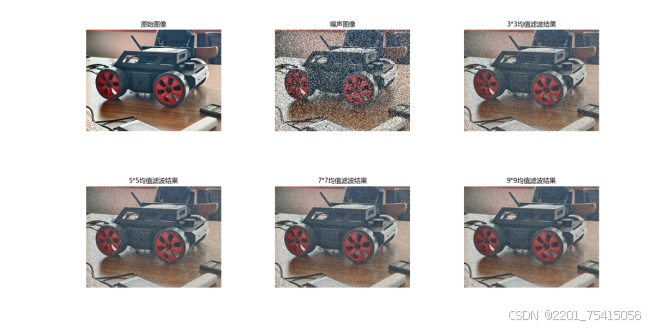
均值滤波：先添加椒盐噪声，再分别进行3*3、5*5、7*7、9*9均值滤波还原，可以看出窗口大小参数越大，对椒盐噪声处理的效果越好。

2.中值滤波

1.代码

function Median_filtering(img)
    figure("中值滤波")
    t = copy(img)
    subplot(1, 3, 1)
    imshow(t)
    t1 = imnoise(t, "salt & pepper", 0.3)
    title("原始图像")
    subplot(1, 3, 2)
    imshow(t1)
    title("加入椒盐噪声后")
    t2 = t
    t2[:, :, 1] = medfilt2(t1[:, :, 1], [3 3])
    t2[:, :, 2] = medfilt2(t1[:, :, 2], [3 3])
    t2[:, :, 3] = medfilt2(t1[:, :, 3], [3 3])
    subplot(1, 3, 3)
    imshow(t2)
    title("中值滤波后")
    tightlayout()
end

2.运行结果

中值滤波：先添加椒盐噪声再通过中值滤波还原，可以看出中值滤波处理椒盐噪声效果比较理想。

3.维纳滤波

1.代码

维纳滤波需要反演，这里对运动模糊后的图像进行维纳滤波复原，但是运动模糊函数在这个版本未兼容（咨询过工程师，应该是笔者的问题，这里采用自编PSF）

#自编补零函数，维纳滤波的前置函数
function pad_psf(PSF, blurredImage)
    # 获取目标大小
    target_rows, target_cols = size(blurredImage)
    psf_rows, psf_cols = size(PSF)

    # 创建补零矩阵
    psf_padded = zeros(target_rows, target_cols)

    # 将PSF嵌入到补零后的矩阵的中心位置
    start_row = div(target_rows - psf_rows, 2) + 1
    start_col = div(target_cols - psf_cols, 2) + 1
    psf_padded[start_row:start_row+psf_rows-1, start_col:start_col+psf_cols-1] .= PSF
    return psf_padded
end

同样，维纳滤波未兼容，这里采用自定义实现函数功能：

# deconvwnr_custom: 维纳反卷积的自定义实现
function deconvwnr_custom(blurredImage, PSF, NSR)
    #   blurredImage: 输入的被模糊的图像（或信号）
    #   PSF: 点扩散函数（Point Spread Function），表示模糊的方式
    #   NSR: 噪声功率与信号功率之比（Noise-to-Signal Ratio）

    # 使用 pad_psf 函数对 PSF 进行补零
    PSF_padded = pad_psf(PSF, blurredImage)

    # 对 PSF 使用 fftshift 将其中心移动到图像的中心
    PSF_padded_shifted = fftshift(PSF_padded)

    # 将输入的图像和补零后的 PSF 转换为频域
    G = fft(blurredImage)
    H = fft(PSF_padded_shifted)

    # 构建维纳滤波器的频域表示
    # 维纳反卷积公式： F_hat = G .* conj(H) ./ (|H|.^2 + NSR)
    H_conj = conj(H)
    H_abs_squared = abs.(H) .^ 2
    Wiener_filter = H_conj ./ (H_abs_squared .+ NSR)

    # 在频域中应用维纳滤波器
    F_hat = G .* Wiener_filter

    # 对结果使用 ifftshift 还原频谱
    F_hat_shifted = ifftshift(F_hat)

    # 转换回空域得到最终结果
    return real(ifft(F_hat_shifted))
end

然后通过调用以上两个函数来实现：

function Wiener_filtering(I)
    img=copy(I)
    figure("维纳滤波")
    subplot(2, 3, 1)
    imshow(img)
    title("原始图像")

    # 转换为双精度图像
    img = im2double(img)
    double_pic = im2double(img)
    # 设置运动模糊参数
    len = 21     # 模糊长度
    theta = 11   # 模糊角度

    # 手动生成运动模糊点扩展函数 (PSF)
    PSF = zeros(len, len)
    mid = ceil(len / 2)
    # 计算模糊方向
    for i = 1:len
        x = Int64(round(mid + (i - mid) * cosd(theta)))
        y = Int64(round(mid + (i - mid) * sind(theta)))
        if x > 0 && x <= len && y > 0 && y <= len
            PSF[y, x] = 1
        end
    end
    # 归一化 PSF
    PSF = PSF / sum(PSF[:])

    # 显示生成的 PSF
    subplot(2, 3, 2)
    imshow(PSF)
    title("自编归一化PSF图像")

    # 对图像进行运动模糊 (逐通道处理)
    blurred_img = img # 创建一个相同大小的副本
    for channel = 1:3
        blurred_img[:, :, channel] = imfilter(img[:, :, channel], PSF; pad="circular", method="conv")
    end
    subplot(2, 3, 3)
    imshow(blurred_img)
    title("运动模糊图像")

    # 添加高斯噪声
    noisy_blurred_img = imnoise(blurred_img, "gaussian", 0, 0.01) # 高斯噪声的均值为 0，方差为 0.01
    subplot(2, 3, 4)
    imshow(noisy_blurred_img)
    title("带高斯噪声的模糊图像")

    restore_ignore_noise = similar(noisy_blurred_img)
    for channel in 1:3
        restore_ignore_noise[:, :, channel] = deconvwnr_custom(noisy_blurred_img[:, :, channel], PSF, 0.000001)#忽视噪声
    end
    subplot(2, 3, 5)
    imshow(restore_ignore_noise), title("忽视噪声维纳滤波图像")


    # 估计噪声功率与信号功率的比值
    signal_var = var(double_pic[:])
    noise_var = 0.01 #方差为0.01的高斯噪声
    estimate_nsr = noise_var / signal_var   #噪信比估值
    # 对每个通道进行维纳滤波复原
    restored_img = similar(noisy_blurred_img)
    for channel in 1:3
        restored_img[:, :, channel] = deconvwnr_custom(noisy_blurred_img[:, :, channel], PSF, estimate_nsr)
    end

    # 显示复原后的图像
    subplot(2, 3, 6)
    imshow(restored_img), title("考虑噪声维纳滤波图像")
    tightlayout()
end

2.运行结果

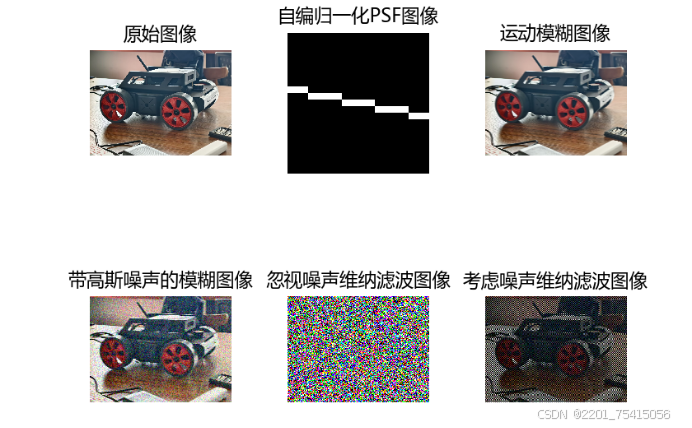
维纳滤波：(P6在复制图像时出现bug，放大播放即可消除)由于MWORKS syslab2024b版本bug，运动模糊函数以及维纳滤波函数无法使用，这里首先通过自编函数实现运动模糊
再添加高斯噪声，再通过自编维纳滤波进行了不考虑信噪比和考虑信噪比的情况下的滤波。

4.小波变换

1.代码

小波变换与MATLAB不同的地方在于MWORKS2024b版本UInt函数不能强制类型转换，这里采用自编函数的形式

#由于MWORKS中的UInt不具备强制转换功能，这里编写Ur函数代替UInt8函数
#为小波变换的前置函数
function Ur(x)
    return UInt8(clamp(round(x), 0, 255))
end

函数主体部分

function Wavelet_transform(I)
    img=copy(I);
    gray_img = rgb2gray(img);
    # 显示灰度图像
    figure("图像预处理");
    subplot(121);
    imshow(img);
    title("原始图像");
    subplot(122);
    imshow(gray_img);
    title("灰度图像");
    
    LoD, HiD = wfilters("haar", "d")
    # 小波变换 (使用单层离散小波变换)
    cA, cH, cV, cD = dwt2(gray_img, LoD, HiD; extmode="symh");
    tt = normalize.(cA);
    # 显示小波变换后的各个子带
    figure("小波变换");
    subplot(2, 2, 1);
    imshow(Ur.(cA));
    title("近似系数");
    
    subplot(2, 2, 2);
    imshow(Ur.(cH));
    title("水平细节系数");
    
    subplot(2, 2, 3);
    imshow(Ur.(cV));
    title("垂直细节系数");
    
    subplot(2, 2, 4);
    imshow(Ur.(cD));
    title("对角线细节系数");
    
    # 小波逆变换
    reconstructed_img = idwt2(cA, cH, cV, cD, "haar");
    
    # 显示小波逆变换后的图像
    figure("小波变换后");
    subplot(221);
    imshow(Ur.(reconstructed_img));
    title("小波逆变换后的重建图像");
    
    # 应用不同的阈值处理 (阈值为20, 50, 100)
    thresh_values = [20, 50, 100];
    
    
    for i = 1:length(thresh_values)
        thresh = thresh_values[i]
    
        # 对小波系数应用阈值处理
        cA_thresh = wthresh(cA, "s", thresh)
        cH_thresh = wthresh(cH, "s", thresh)
        cV_thresh = wthresh(cV, "s", thresh)
        cD_thresh = wthresh(cD, "s", thresh)
    
        # 使用阈值处理后的系数进行小波逆变换
        img_thresh = idwt2(cA_thresh, cH_thresh, cV_thresh, cD_thresh, "haar")
    
        # 显示阈值处理后的图像
        subplot(2, 2, i + 1)
        imshow(Ur.(img_thresh))
        str_c = @sprintf("%d", thresh)
        title("阈值为 " * str_c * "的重建图像")
    
        # title("带阈值的重建图像  阈值为",thresh);
    end
    
end

2.运行结果

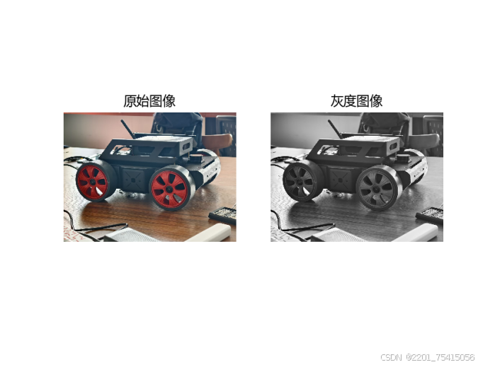
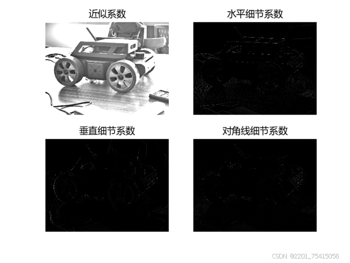
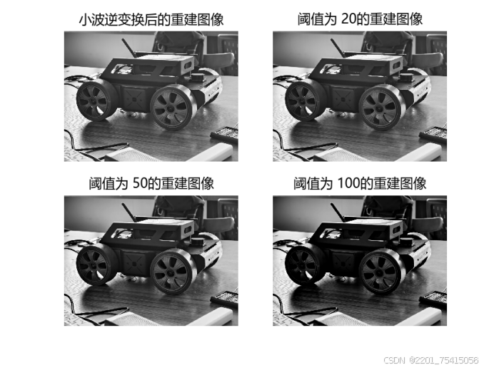
小波变换：首先对图像进行预处理，把彩色图像转为灰度图，再进行单层小波变换(这里使用自编函数Ur进行强制转换)，绘制出近似系数、水平细节系数、垂直细节系数、对角线细节系数，再进行小波逆变换并绘制出复原图像，接着对小波系数进行阈值处理，分别绘制出阈值为20,50,100的重建图像。

5.离散余弦(DCT)变换

1.代码

function Discrete_cosine_transform(I)
    img=copy(I)
    figure("DCT变换")
    subplot(221)
    imshow(img)
    title("原输入图像")
    grayImage = rgb2gray(img)#如果读入的是彩色图像则转化为灰度图像（灰度图像省略这一步） 
    subplot(222)
    imshow(grayImage)
    title("原输入彩色图像转化为灰度图像")
    #对图像DCT变换  
    dctgrayImage = dct(grayImage)
    subplot(223)
    imshow(log.(abs.(dctgrayImage)), [])
    title("DCT变换灰度图像")
    colormap(gray(4))
    colorbar
    #对灰度矩阵进行量化
    dctgrayImage[abs.(dctgrayImage).<0.1] .= 0
    #DCT逆变换  
    I = idct(dctgrayImage) / 255
    subplot(224)
    imshow(I)
    title("经过DCT变换，然后逆变换的灰度图像")
    #对比变换傅里叶变换前后的图像  
    figure("DCT变换前后对比")
    subplot(121)
    imshow(grayImage)
    title("原灰度图像")
    subplot(122)
    imshow(I)
    title("DCT逆变换图像")

end

2.运行结果

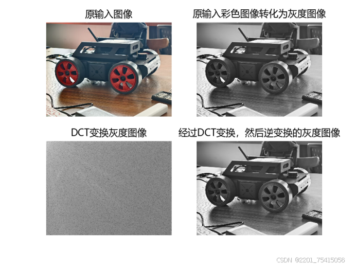
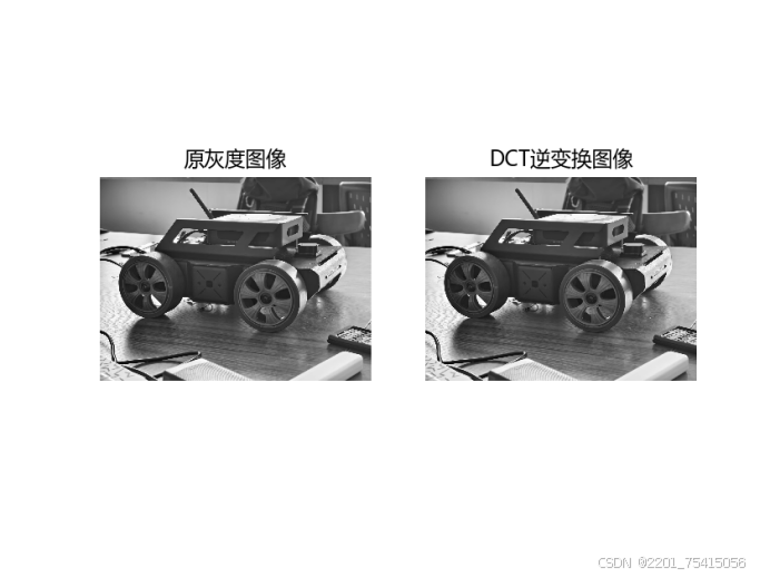
DCT：对输入图像转换为灰度图，进行DCT变换后再进行DCT逆变换，最后将原灰度图像与DCT逆变换图像进行比对。

6.图像傅里叶变换(FFT)变换

1.代码

function Fourier_transform(I)
    img=copy(I)
    image = rgb2gray(img)
    image = im2double(image)
    F_image = fft(image)

    figure("FFT处理图一")
    subplot(221)
    imshow(image)
    title("原始图像")
    subplot(222)
    imshow(abs.(F_image))
    title("幅频响应")
    subplot(223)
    imshow(angle.(F_image))
    title("相频响应")
    subplot(224)
    imshow(fftshift(abs.(F_image)))
    title("频域中心化")
    tightlayout()
    F_imageAfterCentral = fftshift(F_image)
    figure("FFT处理图二")
    subplot(131)
    originalRecoverImage = abs.(ifft(ifftshift(F_imageAfterCentral)))
    imshow(originalRecoverImage)
    title("IFT复原图像")
    # 将四边取0(即将中心化后的中心点取0)
    subplot(132)
    F_imageAfterCentral_m = F_imageAfterCentral
    F_imageAfterCentral_m[280:300, 280:300] .= 0
    imshow(abs.(ifft(ifftshift(F_imageAfterCentral_m))))
    title("中心区域小部分置零")
    subplot(133)
    F_imageAfterCentral_m1 = F_imageAfterCentral
    F_imageAfterCentral_m2 = F_imageAfterCentral
    F_imageAfterCentral_m1[280:300, 280:300] .= 0
    F_difference = F_imageAfterCentral_m2 - F_imageAfterCentral_m1
    imshow(abs.(ifft(ifftshift(F_difference))))
    title("除了中心区域全部置零")
    tightlayout()
end

2.运行结果

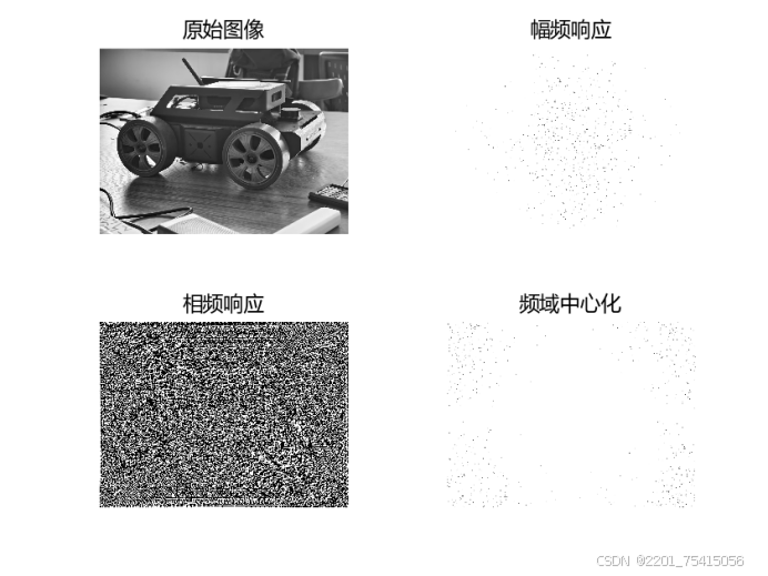
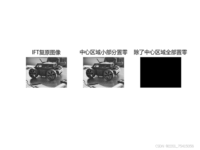
FFT：将彩色图像转换为灰度图像进行运算，绘制出fft变换后的幅频响应和相频响应，并把零频分量移到中心位置，接着绘制出IFT复原图像，以及频域中心区域置零图像、除中心区域外置零图像。可以看出图像细节主要集中在高频区域。

7.完整代码

using  TyImages

#为了形式的规整，这里把读取图像，保存图像封装为自编函数，显示图像被分割到了具体实现的模块中
# 读取图像文件
function open_image(image_path)
    img = imread(image_path)
    return img
end

#自编补零函数，维纳滤波的前置函数
function pad_psf(PSF, blurredImage)
    # 获取目标大小
    target_rows, target_cols = size(blurredImage)
    psf_rows, psf_cols = size(PSF)

    # 创建补零矩阵
    psf_padded = zeros(target_rows, target_cols)

    # 将PSF嵌入到补零后的矩阵的中心位置
    start_row = div(target_rows - psf_rows, 2) + 1
    start_col = div(target_cols - psf_cols, 2) + 1
    psf_padded[start_row:start_row+psf_rows-1, start_col:start_col+psf_cols-1] .= PSF
    return psf_padded
end

# deconvwnr_custom: 维纳反卷积的自定义实现
function deconvwnr_custom(blurredImage, PSF, NSR)
    #   blurredImage: 输入的被模糊的图像（或信号）
    #   PSF: 点扩散函数（Point Spread Function），表示模糊的方式
    #   NSR: 噪声功率与信号功率之比（Noise-to-Signal Ratio）

    # 使用 pad_psf 函数对 PSF 进行补零
    PSF_padded = pad_psf(PSF, blurredImage)

    # 对 PSF 使用 fftshift 将其中心移动到图像的中心
    PSF_padded_shifted = fftshift(PSF_padded)

    # 将输入的图像和补零后的 PSF 转换为频域
    G = fft(blurredImage)
    H = fft(PSF_padded_shifted)

    # 构建维纳滤波器的频域表示
    # 维纳反卷积公式： F_hat = G .* conj(H) ./ (|H|.^2 + NSR)
    H_conj = conj(H)
    H_abs_squared = abs.(H) .^ 2
    Wiener_filter = H_conj ./ (H_abs_squared .+ NSR)

    # 在频域中应用维纳滤波器
    F_hat = G .* Wiener_filter

    # 对结果使用 ifftshift 还原频谱
    F_hat_shifted = ifftshift(F_hat)

    # 转换回空域得到最终结果
    return real(ifft(F_hat_shifted))
end

#由于MWORKS中的UInt不具备强制转换功能，这里编写Ur函数代替UInt8函数
#为小波变换的前置函数
function Ur(x)
    return UInt8(clamp(round(x), 0, 255))
end

function Median_filtering(img)
    figure("中值滤波")
    t = copy(img)
    subplot(1, 3, 1)
    imshow(t)
    t1 = imnoise(t, "salt & pepper", 0.3)
    title("原始图像")
    subplot(1, 3, 2)
    imshow(t1)
    title("加入椒盐噪声后")
    t2 = t
    t2[:, :, 1] = medfilt2(t1[:, :, 1], [3 3])
    t2[:, :, 2] = medfilt2(t1[:, :, 2], [3 3])
    t2[:, :, 3] = medfilt2(t1[:, :, 3], [3 3])
    subplot(1, 3, 3)
    imshow(t2)
    title("中值滤波后")
    tightlayout()
end

function Mean_filtering(I)
    img=copy(I)
    figure("均值滤波")
    subplot(2, 3, 1)
    imshow(img)
    title("原始图像")
    J = imnoise(img, "salt & pepper", 0.3)
    subplot(2, 3, 2)
    imshow(J)
    title("噪声图像")

    H3 = fspecial("average", 3)
    H5 = fspecial("average", 5)
    H7 = fspecial("average", 7)
    H9 = fspecial("average", 9)

    # 利用滤波对图像进行处理
    r3 = imfilter(img, H3)#3*3
    r5 = imfilter(img, H5)#5*5
    r7 = imfilter(img, H7)#7*7
    r9 = imfilter(img, H9)#9*9

    #展示结果
    subplot(2, 3, 3)
    imshow(r3)
    title("3*3均值滤波结果")
    subplot(2, 3, 4)
    imshow(r5)
    title("5*5均值滤波结果")
    subplot(2, 3, 5)
    imshow(r7)
    title("7*7均值滤波结果")
    subplot(2, 3, 6)
    imshow(r9)
    title("9*9均值滤波结果")
    tightlayout()

end


function Wiener_filtering(I)
    img=copy(I)
    figure("维纳滤波")
    subplot(2, 3, 1)
    imshow(img)
    title("原始图像")

    # 转换为双精度图像
    img = im2double(img)
    double_pic = im2double(img)
    # 设置运动模糊参数
    len = 21     # 模糊长度
    theta = 11   # 模糊角度

    # 手动生成运动模糊点扩展函数 (PSF)
    PSF = zeros(len, len)
    mid = ceil(len / 2)
    # 计算模糊方向
    for i = 1:len
        x = Int64(round(mid + (i - mid) * cosd(theta)))
        y = Int64(round(mid + (i - mid) * sind(theta)))
        if x > 0 && x <= len && y > 0 && y <= len
            PSF[y, x] = 1
        end
    end
    # 归一化 PSF
    PSF = PSF / sum(PSF[:])

    # 显示生成的 PSF
    subplot(2, 3, 2)
    imshow(PSF)
    title("自编归一化PSF图像")

    # 对图像进行运动模糊 (逐通道处理)
    blurred_img = img # 创建一个相同大小的副本
    for channel = 1:3
        blurred_img[:, :, channel] = imfilter(img[:, :, channel], PSF; pad="circular", method="conv")
    end
    subplot(2, 3, 3)
    imshow(blurred_img)
    title("运动模糊图像")

    # 添加高斯噪声
    noisy_blurred_img = imnoise(blurred_img, "gaussian", 0, 0.01) # 高斯噪声的均值为 0，方差为 0.01
    subplot(2, 3, 4)
    imshow(noisy_blurred_img)
    title("带高斯噪声的模糊图像")

    restore_ignore_noise = similar(noisy_blurred_img)
    for channel in 1:3
        restore_ignore_noise[:, :, channel] = deconvwnr_custom(noisy_blurred_img[:, :, channel], PSF, 0.000001)#忽视噪声
    end
    subplot(2, 3, 5)
    imshow(restore_ignore_noise), title("忽视噪声维纳滤波图像")


    # 估计噪声功率与信号功率的比值
    signal_var = var(double_pic[:])
    noise_var = 0.01 #方差为0.01的高斯噪声
    estimate_nsr = noise_var / signal_var   #噪信比估值
    # 对每个通道进行维纳滤波复原
    restored_img = similar(noisy_blurred_img)
    for channel in 1:3
        restored_img[:, :, channel] = deconvwnr_custom(noisy_blurred_img[:, :, channel], PSF, estimate_nsr)
    end

    # 显示复原后的图像
    subplot(2, 3, 6)
    imshow(restored_img), title("考虑噪声维纳滤波图像")
    tightlayout()
end


function Fourier_transform(I)
    img=copy(I)
    image = rgb2gray(img)
    image = im2double(image)
    F_image = fft(image)

    figure("FFT处理图一")
    subplot(221)
    imshow(image)
    title("原始图像")
    subplot(222)
    imshow(abs.(F_image))
    title("幅频响应")
    subplot(223)
    imshow(angle.(F_image))
    title("相频响应")
    subplot(224)
    imshow(fftshift(abs.(F_image)))
    title("频域中心化")
    tightlayout()
    F_imageAfterCentral = fftshift(F_image)
    figure("FFT处理图二")
    subplot(131)
    originalRecoverImage = abs.(ifft(ifftshift(F_imageAfterCentral)))
    imshow(originalRecoverImage)
    title("IFT复原图像")
    # 将四边取0(即将中心化后的中心点取0)
    subplot(132)
    F_imageAfterCentral_m = F_imageAfterCentral
    F_imageAfterCentral_m[280:300, 280:300] .= 0
    imshow(abs.(ifft(ifftshift(F_imageAfterCentral_m))))
    title("中心区域小部分置零")
    subplot(133)
    F_imageAfterCentral_m1 = F_imageAfterCentral
    F_imageAfterCentral_m2 = F_imageAfterCentral
    F_imageAfterCentral_m1[280:300, 280:300] .= 0
    F_difference = F_imageAfterCentral_m2 - F_imageAfterCentral_m1
    imshow(abs.(ifft(ifftshift(F_difference))))
    title("除了中心区域全部置零")
    tightlayout()
end


function Discrete_cosine_transform(I)
    img=copy(I)
    figure("DCT变换")
    subplot(221)
    imshow(img)
    title("原输入图像")
    grayImage = rgb2gray(img)#如果读入的是彩色图像则转化为灰度图像（灰度图像省略这一步） 
    subplot(222)
    imshow(grayImage)
    title("原输入彩色图像转化为灰度图像")
    #对图像DCT变换  
    dctgrayImage = dct(grayImage)
    subplot(223)
    imshow(log.(abs.(dctgrayImage)), [])
    title("DCT变换灰度图像")
    colormap(gray(4))
    colorbar
    #对灰度矩阵进行量化
    dctgrayImage[abs.(dctgrayImage).<0.1] .= 0
    #DCT逆变换  
    I = idct(dctgrayImage) / 255
    subplot(224)
    imshow(I)
    title("经过DCT变换，然后逆变换的灰度图像")
    #对比变换傅里叶变换前后的图像  
    figure("DCT变换前后对比")
    subplot(121)
    imshow(grayImage)
    title("原灰度图像")
    subplot(122)
    imshow(I)
    title("DCT逆变换图像")

end

function Wavelet_transform(I)
    img=copy(I);
    gray_img = rgb2gray(img);
    # 显示灰度图像
    figure("图像预处理");
    subplot(121);
    imshow(img);
    title("原始图像");
    subplot(122);
    imshow(gray_img);
    title("灰度图像");
    
    LoD, HiD = wfilters("haar", "d")
    # 小波变换 (使用单层离散小波变换)
    cA, cH, cV, cD = dwt2(gray_img, LoD, HiD; extmode="symh");
    tt = normalize.(cA);
    # 显示小波变换后的各个子带
    figure("小波变换");
    subplot(2, 2, 1);
    imshow(Ur.(cA));
    title("近似系数");
    
    subplot(2, 2, 2);
    imshow(Ur.(cH));
    title("水平细节系数");
    
    subplot(2, 2, 3);
    imshow(Ur.(cV));
    title("垂直细节系数");
    
    subplot(2, 2, 4);
    imshow(Ur.(cD));
    title("对角线细节系数");
    
    # 小波逆变换
    reconstructed_img = idwt2(cA, cH, cV, cD, "haar");
    
    # 显示小波逆变换后的图像
    figure("小波变换后");
    subplot(221);
    imshow(Ur.(reconstructed_img));
    title("小波逆变换后的重建图像");
    
    # 应用不同的阈值处理 (阈值为20, 50, 100)
    thresh_values = [20, 50, 100];
    
    
    for i = 1:length(thresh_values)
        thresh = thresh_values[i]
    
        # 对小波系数应用阈值处理
        cA_thresh = wthresh(cA, "s", thresh)
        cH_thresh = wthresh(cH, "s", thresh)
        cV_thresh = wthresh(cV, "s", thresh)
        cD_thresh = wthresh(cD, "s", thresh)
    
        # 使用阈值处理后的系数进行小波逆变换
        img_thresh = idwt2(cA_thresh, cH_thresh, cV_thresh, cD_thresh, "haar")
    
        # 显示阈值处理后的图像
        subplot(2, 2, i + 1)
        imshow(Ur.(img_thresh))
        str_c = @sprintf("%d", thresh)
        title("阈值为 " * str_c * "的重建图像")
    
        # title("带阈值的重建图像  阈值为",thresh);
    end
    
end


function main()
    img=open_image("a1.jpg")
    Median_filtering(img)
    Mean_filtering(img)
    Wiener_filtering(img)
    Fourier_transform(img)
    Discrete_cosine_transform(img)
    Wavelet_transform(img)
    
end
    
main()