| 本文仅应用已训练的模型，不包括方法原理及如何用自己的数据集训练的分享，可参考其他推文；

1. 介绍Hovernet

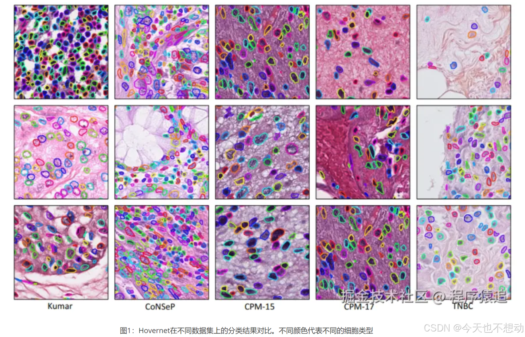
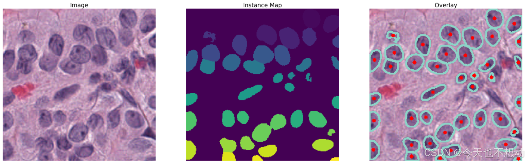
HoverNet是一种基于深度学习的先进网络模型，能够进行细胞核分割与分类，并在原始图像上以颜色叠加的方式直观的展示结果（效果如下所示）。

2. 安装

参考github安装（https://github.com/vqdang/hover_net）

# 参考github安装：PyTorch version 1.6 with CUDA 10.2.
conda env create -f environment.yml
conda activate hovernet
pip install torch==1.6.0 torchvision==0.7.0

# ps：此处pytorch的安装可以参考官网，根据自己的显卡版本安装。

3. Inference

采用官网的检查点进行推断

Step1：代码下载

git clone https://github.com/vqdang/hover_net
cd hover_net

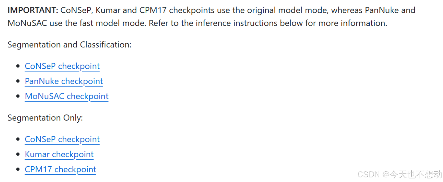
Step2：检查点下载

• 官方检查点所在网址：https://drive.google.com/drive/folders/17IBOqdImvZ7Phe0ZdC5U1vwPFJFkttWp

• 下载检查点并放在hover_net文件夹下
  

不同预训练模型细胞类型展示：

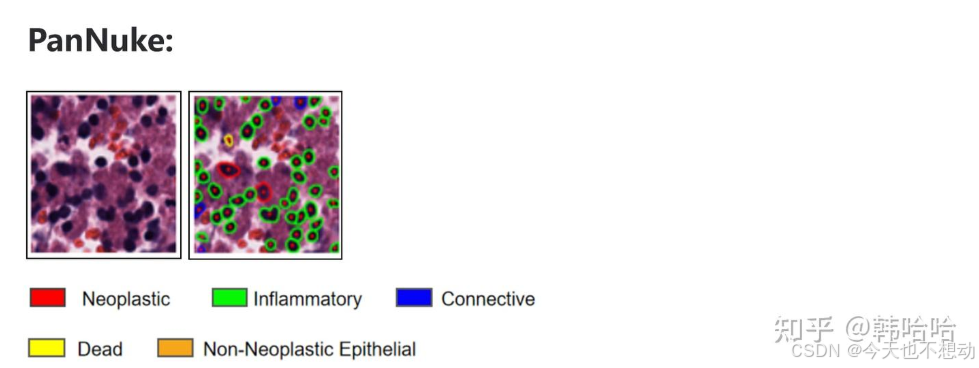
PanNuke:
0:背景(Background)
1:肿瘤 (Neoplastic) - 红色
2:炎症 (Inflammatory)	- 绿色
3:连接(Connective) - 蓝色
4:死亡 (Dead) - 黄色
5：非肿瘤性上皮 (Non-Neoplastic Epithelial) - 橙色


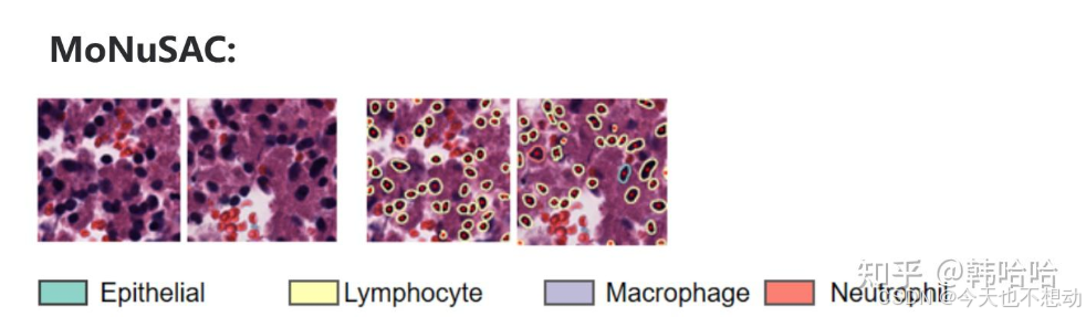
MoNuSAC:
0:背景(Background)
1:上皮(Epithelial) 
2:淋巴细胞(Lymphocyte)	
3:巨噬细胞 (Macrophage)
4:嗜中性粒细胞 (Neutrophil)

Step3：数据准备

• 创建目录input_dataset_tiles，目录下为格式为png ,jpg and tiff的图片。如下所示：

• type_info_pannuke.json/type_info_MoNuSAC.json准备

  • type_info_pannuke.json内容如下:
    {
        "0" : ["nolabe", [0  ,   0,   0]],
        "1" : ["neopla", [255,   0,   0]],
        "2" : ["inflam", [0  , 255,   0]],
        "3" : ["connec", [0  ,   0, 255]],
        "4" : ["necros", [255, 255,   0]],
        "5" : ["no-neo", [255, 165,   0]]
    }
    
    type_info_MoNuSAC.json内容如下:
    {
        "0" : ["nolabe", [0  ,   0,   0]],
        "1" : ["epithelial", [141,   211,   199]],
        "2" : ["Lymphocyte", [255  , 255,   179]],
        "3" : ["Macrophage", [190  ,   186, 218]],
        "4" : ["Neutrophil", [251, 128,   114]]
    }
    Ps: 上述颜色皆可自定义
    

Step4：推断

根据自己的目标选择对应的检查点和json文件

### pannuke
python run_infer.py --gpu='0' --nr_types=6 --type_info_path='type_info_pannuke.json'  --model_path='./hover-net-pytorch-weights/hovernet_fast_pannuke_type_tf2pytorch.tar' --model_mode='fast' --nr_inference_workers=8 --nr_post_proc_workers=16 --batch_size=1  tile --input_dir='./input_dataset_tiles/' --output_dir='./output_tiles_Pannuke/' --mem_usage=0.1 --draw_dot --save_qupath


### MoNuSAC
python run_infer.py --gpu='0' --nr_types=5 --type_info_path='type_info_MoNuSAC.json'  --model_path='./hover-net-pytorch-weights/hovernet_fast_monusac_type_tf2pytorch.tar' --model_mode='fast' --nr_inference_workers=8 --nr_post_proc_workers=16 --batch_size=1  tile --input_dir='./input_dataset_tiles/' --output_dir='./output_tiles_MoNuSAC/' --mem_usage=0.1 --draw_dot --save_qupath

# 根据tile大小可调节mem_usage等参数

Step5：结果解释

以MoNuSAC检查点的输出结果为例，输出目录中包含四个文件夹，分别为overlay（标注细胞类别的图片），mat，qupath和json

• JSON文件: 对于图像块(tiles)和全切片图像，输出包含以下键(keys):

  • bbox:每个细胞核的边界框坐标。

  • centroid:每个细胞核的质心坐标。

  • contour:每个细胞核的轮廓坐标。

  • type_prob:每个细胞核属于各个类别的概率(默认配置不输出此信息)。

  • type:每个细胞核预测的类别。

• MAT文件: 仅图像块输出，包含以下键:

  • raw:网络的原始输出 (默认配置不输出此信息)。
  • inst_map:实例映射，包含从0到N的值，其中N是图像中细胞核的数量
  • inst type:长度为N的列表，包含每个细胞核的预测结果。

• overlay：

  • PNG叠加图，即将细胞核边界叠加在原始RGB图像上，可以直接在原始图像上可视化细胞核的分割和分类结果。

# load the libraries

import sys
sys.path.append('../')

import numpy as np
import pandas as pd
import os
import glob
import matplotlib.pyplot as plt
import scipy.io as sio
import cv2
import json
import openslide

from misc.wsi_handler import get_file_handler
from misc.viz_utils import visualize_instances_dict

tile_path = '../input_dataset_tiles//'
tile_json_path = '../output_tiles_MoNuSAC///json/'
tile_mat_path = '../output_tiles_MoNuSAC///mat/'
tile_overlay_path  = '../output_tiles_MoNuSAC//overlay//'

预测结果图展示

# 结果图展示
# load the original image, the `.mat` file and the overlay
image_list = glob.glob(tile_path + '*.png')
image_list.sort()

# get a random image 
rand_nr = np.random.randint(0,len(image_list))
image_file = image_list[rand_nr]
# image_file = "../input_dataset_tiles/12_TCGA-EY-A1GL_x_49296_y_29696_a_99.967.png"
print(image_file)

basename = os.path.basename(image_file)
image_ext = basename.split('.')[-1]
basename = basename[:-(len(image_ext)+1)]

image = cv2.imread(image_file)
# convert from BGR to RGB
image = cv2.cvtColor(image, cv2.COLOR_BGR2RGB)

# get the corresponding `.mat` file 
result_mat = sio.loadmat(tile_mat_path + basename + '.mat')

# get the overlay
overlay = cv2.imread(tile_overlay_path + basename + '.png')
overlay = cv2.cvtColor(overlay, cv2.COLOR_BGR2RGB)


# plot the original image, along with the instance map and the overlay
plt.figure(figsize=(40,20))

plt.subplot(1,3,1)
plt.imshow(image[:400,:400,:])
plt.axis('off')
plt.title('Image', fontsize=25)

plt.subplot(1,3,2)
plt.imshow(inst_map[:400,:400])
plt.axis('off')
plt.title('Instance Map', fontsize=25)

plt.subplot(1,3,3)
plt.imshow(overlay[:400,:400,:])
plt.axis('off')
plt.title('Overlay', fontsize=25)

plt.show()

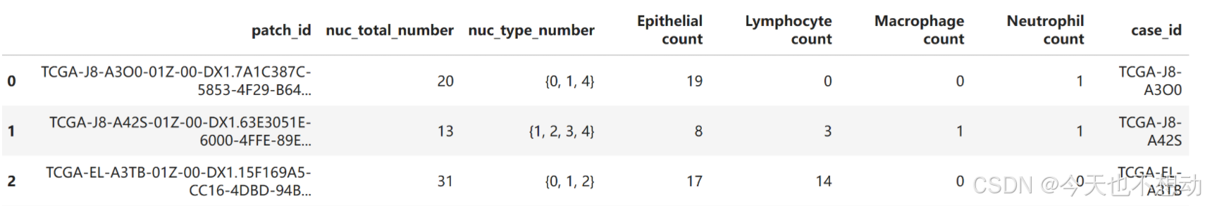
统计每张tile上各种细胞类型的比例

# 假设每张切片（slide）选择了代表性的10个tile进行分析，现统计每张tile上各种细胞类型的比例
def read_json(json_file):
    type_list = []
    type_prob_list = []
    centroid_list = []

    with open(json_file) as json_files:
        data = json.load(json_files)
        mag_info = data['mag']
        nuc_info = data['nuc']
        for inst in nuc_info:
            inst_info = nuc_info[inst]
            inst_centroid = inst_info['centroid']
            centroid_list.append(inst_centroid)
            
            inst_type = inst_info['type']
            type_list.append(inst_type)

            inst_type_prob = inst_info['type_prob']
            type_prob_list.append(inst_type_prob)
    return type_list


from collections import Counter
# 从左到右每列分别代表 patch的名称，patch中的细胞核总数量， patch中的细胞核总数量， 不同类型细胞的数量
df_out = pd.DataFrame(columns = ["patch_id", "nuc_total_number","nuc_type_number","Epithelial count", "Lymphocyte count","Macrophage count","Neutrophil count" ])
json_file_list = os.listdir(tile_json_path)
for json_file_base in json_file_list:
    json_file = tile_json_path + json_file_base
    type_list = read_json(json_file)
    nuc_type_number = set(type_list)
    char_count = Counter(type_list)
    nuc_total_number = char_count[1]+char_count[2]+char_count[3]+char_count[4] 
    df_out.loc[len(df_out)] = [json_file_base.replace(".json",""),nuc_total_number,nuc_type_number, char_count[1],char_count[2],char_count[3],char_count[4] ]
df_out["case_id"] = df_out["patch_id"].str.slice(0,12)
df_out.to_csv("hover-net_celltype_count_inTiles_byMoNuSAC.csv",index=False)
df_out.head()    

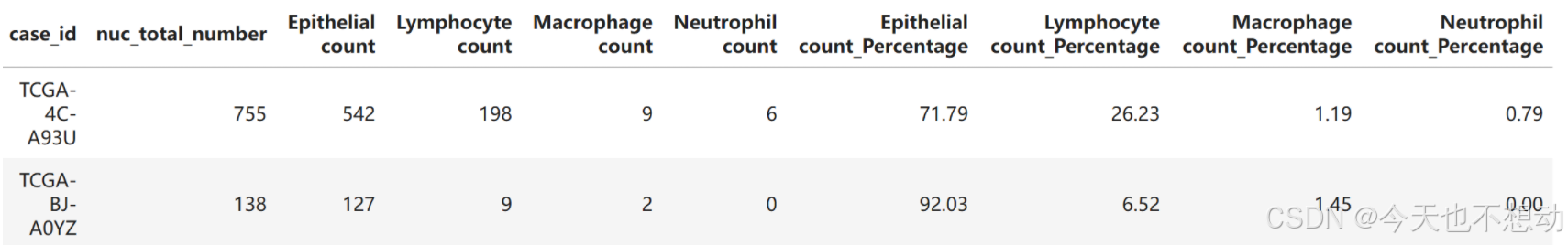
计算每张slide上每种细胞的近似占比

# 计算每张slide上每种细胞的近似占比
df_out_slide = df_out
df_out_slide["case_id"] = df_out_slide["patch_id"].str.slice(0,12)
df_out_slide = df_out_slide.groupby("case_id").agg({'nuc_total_number':"sum",   
       'Epithelial count':"sum", 'Lymphocyte count':"sum", 'Macrophage count':"sum",
       'Neutrophil count':"sum" }).reset_index()

# 计算百分比
percentage_columns = [ "Epithelial count", "Lymphocyte count","Macrophage count","Neutrophil count" ]
for column in percentage_columns:
    df_out_slide[column + '_Percentage'] = round((df_out_slide[column] / df_out_slide['nuc_total_number']) * 100,2)

df_out_slide = df_out_slide.fillna(0)
df_out_slide = df_out_slide[df_out_slide["nuc_total_number"]>10]
df_out_slide.to_csv("hover-net_celltype_count_inSlides_byMoNuSAC.csv",index=False)
df_out_slide.head(2)

4. 应用

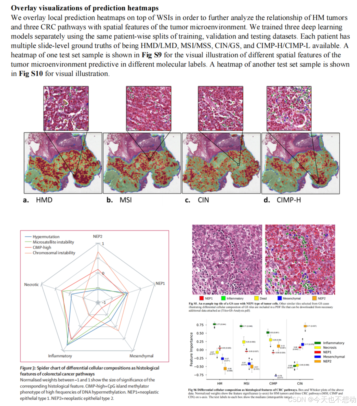
方向一：统计不同分组不同细胞类型的占比及肿瘤浸润淋巴细胞（Tumor-Infiltrating Lymphocytes, TILs）的富集打分

参考文献：Development and validation of a weakly supervised deeplearning framework to predict the status of molecularpathways and key mutations in colorectal cancer fromroutine histologyimages: a retrospective study

参考文献：Interpretable multi-modal artificial intelligence model for predicting gastric cancer response to neoadjuvant chemotherapy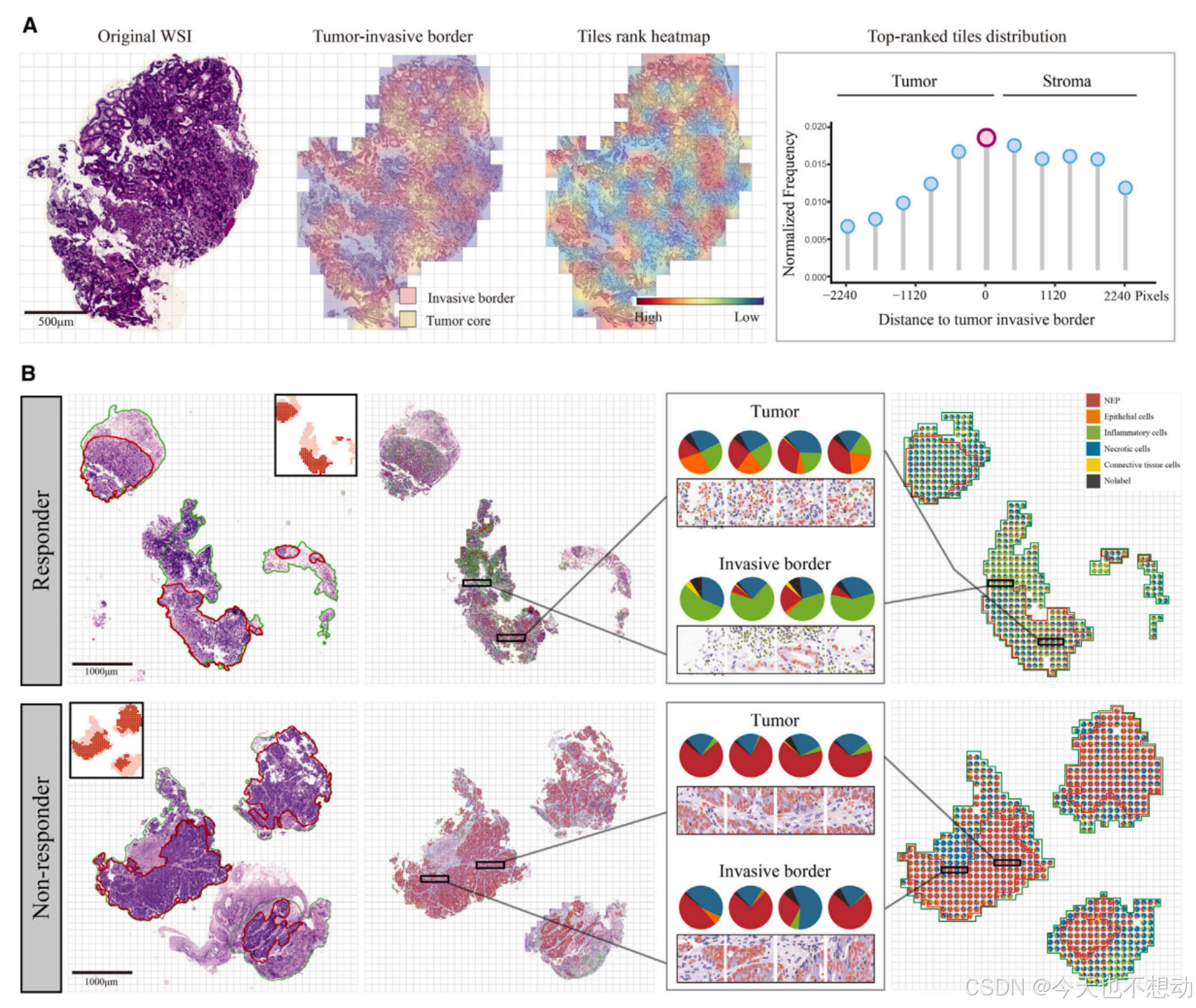


Ps: 肿瘤浸润淋巴细胞（Tumor-Infiltrating Lymphocytes, TILs）的富集打分 = 淋巴细胞核的数量（Nlymph）/ 肿瘤细胞核的数量（Ntumor）; 意义： 高TILs富集通常预示着更好的预后， 更良好的免疫治疗反应。

方向二：统计比较分割细胞的形态学特征

• https://juejin.cn/post/7419148660796342291（收费）
• 直接采用cellprofiers提取核形态学特征，再进行比较；

方向三：基于重要的tile分割图或者WSI 分割图提取特征用于模型构建

参考文献：Development and interpretation of a pathomics-driven ensemble model for predicting the response to immunotherapy in gastric cancer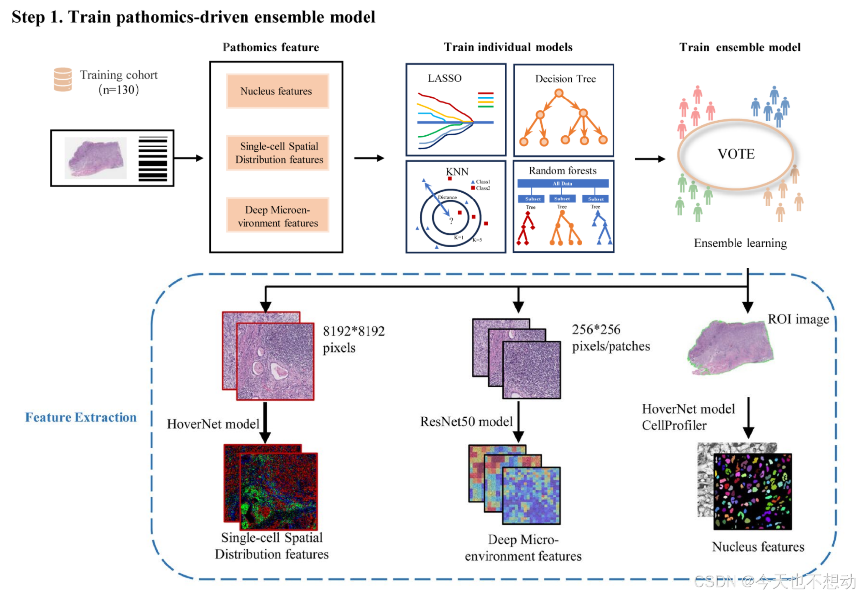

提取三类病理特征如下：

• Pathomics tumor nucleus features：CellProfiler
• Deep microenvironment pathomics features：Image patches of size 256×256 were extracted, without overlap, from all identified tissue regions after segmentation. Subsequently, a pretrained ResNet50 model on ImageNet was used as an encoder to convert each 256×256 patch into a 1024-dimensional feature vector.
  s**：CellProfiler
• Deep microenvironment pathomics features：Image patches of size 256×256 were extracted, without overlap, from all identified tissue regions after segmentation. Subsequently, a pretrained ResNet50 model on ImageNet was used as an encoder to convert each 256×256 patch into a 1024-dimensional feature vector.
• Single-cell spatial distribution pathomics features：For each whole slide image (WSI), a ROI image of size 8192x8192 pixels was cropped at 40x magnification using Openslide. A HoverNet model2 pretrained on the Pannuke dataset was employed to segment and classify cells in the ROI, including tumor cells, lymphocytes, stromal cells, dead cells, and non-neoplastic epithelial cells. The number of tumor cells, lymphocytes, and stromal cells per unit square was computed on a 16x16 μm2 grid to generate an RGB image. In this image, the red, green, and blue channels represent the density maps of tumor cells, lymphocytes, and stromal cells, respectively. The same ResNet50 model used for tumor microenvironment feature extraction was applied to capture different cell types and their spatial organization patterns in the RGB image.