YOLOv10【第十一章:生成式 AI 与自动标注篇·第2节】SAM + YOLOv10 自动标注:从框到 Mask 到标签

🏆 本文收录于 《YOLOv10实战:从入门到深度优化》 专栏。
该专栏系统复现并深度梳理全网主流 YOLOv10 改进方法与工程实战案例,覆盖分类、目标检测、实例分割、多目标追踪、关键点检测、旋转目标检测等多个方向,坚持 持续更新 + 深度解析 + 工程验证。
专栏将围绕 YOLOv10 的网络结构、训练策略、标签分配、损失函数、数据增强、模型压缩、推理加速与部署落地等内容展开,重点分析 Consistent Dual Assignments(一致性双重标签分配)、NMS-Free End-to-End Detection(无 NMS 端到端检测)、Holistic Efficiency-Accuracy Driven Model Design(整体效率-精度驱动模型设计) 等核心设计思想,并结合实际项目讲解其改进方式与应用价值。
部分章节还会结合国内外前沿论文与 AIGC 大模型技术,对主流改进方案进行重构与再设计,使内容更加贴近真实业务场景,适合希望深入研究 YOLOv10 或具有工程落地需求的开发者学习与参考。
🎯限时特惠:当前活动一折秒杀,一次订阅,终身有效,后续所有更新章节全部免费解锁 👉 传送门 👈️
🎉 本专栏还不够过瘾?别急,好戏才刚刚开始!我已经为你准备了一整套 YOLO 进阶实战大礼包🎁:
👉 《YOLOv8实战》
👉 《YOLOv9实战》
👉 《YOLOv10实战》
👉 《YOLOv11实战》
👉 《YOLOv12实战》
👉 以及最新上线的 《YOLOv26实战》想一次搞定所有版本?直接冲 《YOLO全栈实战合集》,一站式涵盖 YOLO 各版本实战教学!
🚀 想学哪个版本?直接找 bug 菌“许愿”,安排!必须安排!🚀
🎯 本文定位:计算机视觉 × YOLOv10 生成式 AI 与自动标注篇
📅 预计阅读时间:约 45~60 分钟
🏷️ 难度等级:⭐⭐⭐⭐☆(高级)
🔧 技术栈:Python 3.9+ · PyTorch 2.0+ · YOLOv10 · ByteTrack · OpenCV · NumPy
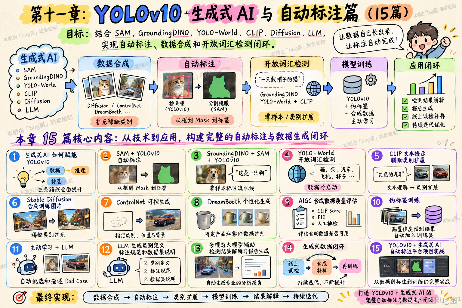
全文目录:
- 📌 上期回顾
- 🎯 本节主题:SAM + YOLOv10 自动标注:从框到 Mask 到标签
- 📌 本节总结
- 🔮 下期预告:GroundingDINO + SAM + YOLOv10 零样本标注流水线
- 📌 附录
- 🧧🧧 文末福利,等你来拿!🧧🧧
- 👨💻 About Me · 关于作者
写在前面:如果你跟着这个专栏一路走来,应该对"数据是模型的粮食"这句话有越来越深的体感了。上一节我们聊了生成式 AI 赋能 YOLOv10 的三条路线,算是打开了一扇大门。这一节,我们要走进门里,动手搭建第一条真正意义上的自动标注流水线——SAM + YOLOv10 联合标注方案。这条路线我自己踩过不少坑,也有一些让我拍大腿的"原来如此"时刻,都会在文章里跟你分享。
📌 上期回顾
在上期《》内容中,我们系统梳理了生成式 AI 介入 YOLOv10 训练体系的三条核心路线,这里做一个简要回顾,方便你建立知识连贯性。
路线一:数据生成路线。 当你面临某个类别样本严重不足的问题时,Stable Diffusion、DALL·E 等图像生成模型可以凭借文本提示(Prompt)批量合成目标图片。这条路线解决的是"没有数据"的问题,属于数据侧的扩充手段。
路线二:自动标注路线。 数据有了,但标注工作依然繁重。SAM(Segment Anything Model)、GroundingDINO、YOLO-World 等模型可以辅助甚至全自动完成标注任务——框的定位、像素级分割、类别语义对齐,都可以由 AI 协助完成。这条路线解决的是"有数据但没标签"的问题。
路线三:推理增强路线。 在模型部署阶段,CLIP、LLM、多模态大模型可以辅助解释检测结果、扩展识别类别边界、生成可读性报告。这条路线解决的是"模型能用但用得不够好"的问题。
三条路线本质上对应了一个完整的 AI 工程闭环:生成数据 → 生成标签 → 增强推理。上一节我们重点讲了整体框架和思想,这一节我们深入第二条路线,把 SAM 和 YOLOv10 联合自动标注这件事讲透、讲细、讲到你能直接动手实操。
🎯 本节主题:SAM + YOLOv10 自动标注:从框到 Mask 到标签
一、为什么标注是 AI 工程里最痛的环节
做过工业落地项目的工程师大概都有这样的经历:模型训练本身花了三天,数据标注却花了三个星期。这不是夸张,而是很多项目的真实写照。
传统的目标检测标注流程大致是这样的:人工打开标注工具(LabelImg、LabelMe、CVAT 等),对每一张图逐个画框,然后为每个框选择类别标签,最后导出 YOLO 格式的 .txt 标注文件。这个过程的每一步都依赖人工判断,效率低、成本高、质量也因人而异。
一个经验丰富的标注员,每小时大概能完成 200~500 个高质量框标注。如果你有 10 万张图,每张平均 5 个目标,那就是 50 万个框——需要 1000~2500 个工时,折合至少几十个工作日。这还不算返工和质检的成本。
更头疼的问题是:某些场景的标注本身需要专业知识。医学影像、工业缺陷、卫星遥感……不是随便找个人坐下来画框就能完成的,需要专业背景才能判断"这块区域算不算缺陷"、“这个细胞核要不要圈进去”。
SAM 的出现,正是在这个痛点上打开了一道缺口。
二、SAM 是什么:从"点一下"到"分割一切"
2.1 SAM 的诞生背景
2023 年 4 月,Meta AI 发布了 Segment Anything Model(SAM),这个名字本身就是一个宣言——“分割任何东西”。不是"分割某些东西",不是"在特定数据集上分割",而是"任何"。
SAM 的论文标题是《Segment Anything》,配套发布了 SA-1B 数据集,包含超过 1100 万张图像和 10 亿个掩码(Mask)。这个数据集的体量本身就说明了 SAM 训练时所调动的资源规模。
SAM 的核心能力可以用一句话描述:给定任意形式的提示(点、框、文字、掩码),在任意图像上生成高质量的分割掩码。
这里的"任意提示"是 SAM 最关键的设计哲学。不同于过去的分割模型需要针对特定类别进行训练,SAM 是一个**提示驱动(Prompt-driven)**的通用分割器,它不在乎你要分割的是猫、是零件、还是一片叶子——只要你给它一个"线索",它就能完成分割。
2.2 SAM 的模型架构
SAM 的架构由三个核心模块组成,理解这三个模块,是后续正确使用 SAM 的基础。
相关示意图绘制如下,仅供参考:
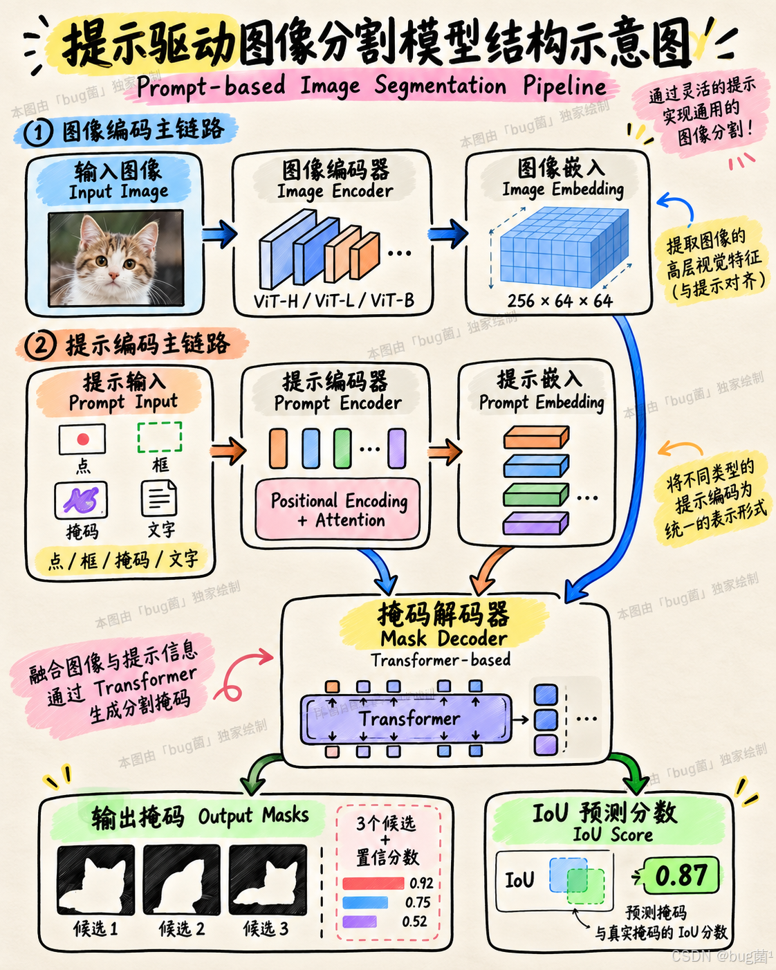
图像编码器(Image Encoder):SAM 使用 Vision Transformer(ViT)作为图像编码器,有三个规格:ViT-H(最大,最准确)、ViT-L(中等)、ViT-B(最小,速度最快)。图像被预处理为 1024×1024 分辨率,经过编码器后输出 256×64×64 的图像嵌入张量。重要的是:图像嵌入只需要计算一次,可以缓存复用,这对批量标注场景至关重要——你可以对同一张图使用不同的提示多次查询,只需要一次图像编码。
提示编码器(Prompt Encoder):接收各种形式的提示输入。点提示通过位置编码处理;框提示被表示为两个角点坐标;掩码提示通过卷积下采样;文字提示(SAM 原版不支持,但 Grounded-SAM 扩展了这个能力)通过 CLIP 文本编码器处理。
掩码解码器(Mask Decoder):这是 SAM 最轻量的模块,基于 Transformer 设计,将图像嵌入和提示嵌入融合后,输出三个候选掩码(对应目标的整体、部分、局部三种粒度)以及每个掩码的 IoU 置信分数。
2.3 SAM2:进化与升级
2024 年,Meta 发布了 SAM2(Segment Anything Model 2),在原版 SAM 的基础上做了重要升级:
- 支持视频分割(时序一致性追踪)
- 引入了流式记忆机制(Streaming Memory)
- 推理速度更快,精度更高
- 模型权重更小(相同精度下)
在本节的实战代码中,我们会同时演示 SAM 和 SAM2 的使用,你可以根据自己的环境选择。
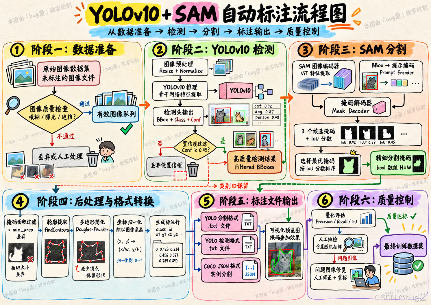
三、YOLOv10 检测框 + SAM 分割的联合逻辑
理解了 SAM 的能力后,我们来思考一个核心问题:SAM 能生成分割掩码,但它不知道"这是什么类别"。YOLOv10 能检测目标并预测类别,但它只输出边界框(Bounding Box),不提供像素级的精细分割。两者如何协同?
这正是 SAM + YOLOv10 联合标注方案的核心思想:YOLOv10 负责"在哪里,是什么"(定位 + 分类),SAM 负责"精确到哪个像素"(精细分割)。
整个流水线的逻辑如下,仅供参考:
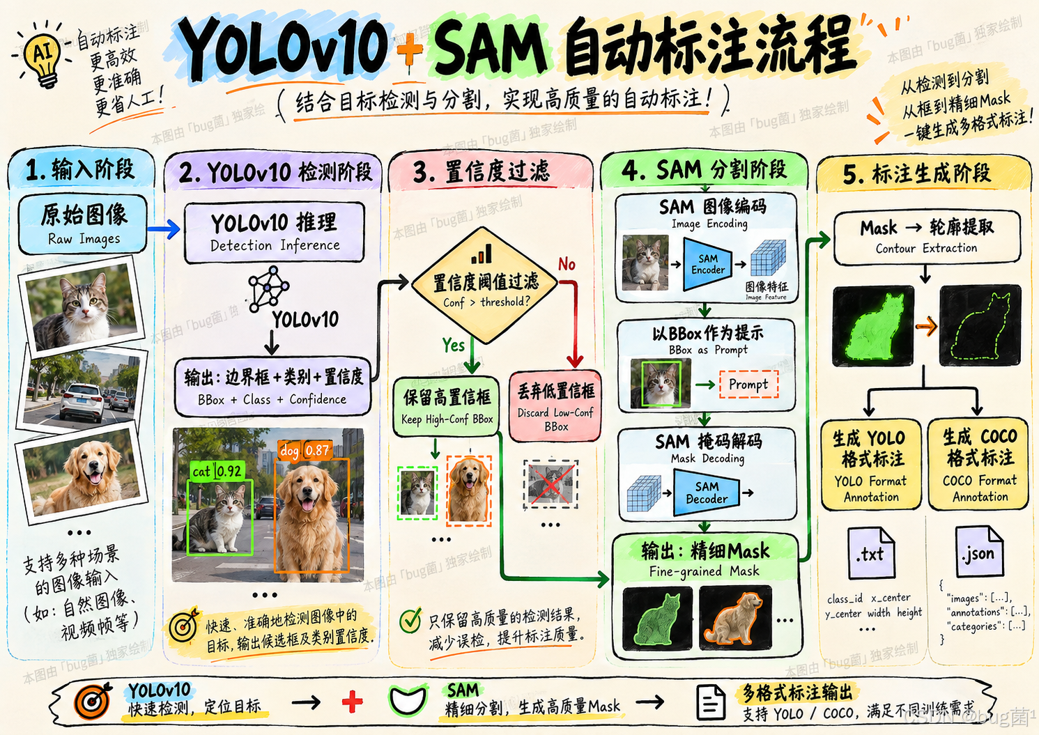
这个流程的精妙之处在于:YOLOv10 的检测框既是分类的依据,也是 SAM 的提示(Prompt)。SAM 的框提示功能非常适合这个场景——你给它一个边界框,它就在这个框的范围内寻找最合适的分割掩码。这样,两个模型各司其职,相互补充,最终产出的是带有类别标签的精细掩码标注,既可用于实例分割训练,也可转化为矩形框标注用于检测训练。
四、数据格式深度解析:YOLO 与 COCO 的标注规范
在动手写代码之前,我们必须把标注数据的格式搞清楚。很多人在这一步栽跟头,生成了标注文件却发现训练时报错——往往是格式细节出了问题。
4.1 YOLO 检测格式(.txt)
YOLO 检测任务的标注文件是 .txt 格式,每行代表一个目标,格式如下:
<class_id> <x_center> <y_center> <width> <height>
所有坐标值均已归一化(除以图像宽度或高度),取值范围 [0, 1]。例如:
0 0.5234 0.3821 0.1245 0.2156
1 0.7823 0.6543 0.0987 0.1432
第一行表示类别 0 的目标,中心点在 (0.5234, 0.3821),宽度 0.1245,高度 0.2156。
4.2 YOLO 分割格式(.txt)
YOLO 分割任务的标注文件也是 .txt 格式,但每行的格式不同:
<class_id> <x1> <y1> <x2> <y2> ... <xn> <yn>
每行包含一个类别 ID,后跟若干归一化的多边形顶点坐标对。顶点数量不固定(通常 6~100 个点),代表目标轮廓的多边形近似。
0 0.512 0.345 0.523 0.412 0.498 0.445 0.487 0.398
4.3 COCO 实例分割格式(.json)
COCO 格式使用 JSON 文件,结构更复杂但表达能力更强。掩码可以用 segmentation 字段的多边形列表表示,也可以用 RLE(Run-Length Encoding)压缩编码表示。
{
  "annotations": [
    {
      "id": 1,
      "image_id": 1,
      "category_id": 1,
      "segmentation": [[512.3, 345.1, 523.8, 412.6, ...]],
      "area": 1234.56,
      "bbox": [480.0, 320.0, 120.0, 150.0],
      "iscrowd": 0
    }
  ]
}
理解了这三种格式,我们在代码里生成标注时就有了明确的目标。
五、环境搭建:把工具都装好
工欲善其事,必先利其器。我们先把需要的库和模型权重都准备好。
# ============================================================
# 环境依赖安装命令(在终端执行,非 Python 代码)
# ============================================================

# 安装 ultralytics(包含 YOLOv10 和 SAM2 支持)
# pip install ultralytics>=8.3.0

# 安装 segment-anything(Meta 原版 SAM)
# pip install git+https://github.com/facebookresearch/segment-anything.git

# 安装 SAM2(推荐使用更新版本)
# pip install git+https://github.com/facebookresearch/sam2.git

# 安装其他依赖
# pip install opencv-python numpy Pillow matplotlib tqdm pycocotools

# ============================================================
# 模型权重下载(Python 代码,可直接执行)
# ============================================================

import os
import urllib.request

def download_weights(url, save_path):
    """
    下载模型权重文件
    Args:
        url: 下载链接
        save_path: 本地保存路径
    """
    if os.path.exists(save_path):
        print(f"[跳过] 权重文件已存在: {save_path}")
        return

    print(f"[下载] 正在下载: {os.path.basename(save_path)}")
    os.makedirs(os.path.dirname(save_path), exist_ok=True)

    # 使用 urllib 下载,显示进度
    def reporthook(count, block_size, total_size):
        percent = int(count * block_size * 100 / total_size)
        print(f"\r  进度: {percent}%", end="", flush=True)

    urllib.request.urlretrieve(url, save_path, reporthook)
    print(f"\n[完成] 已保存至: {save_path}")

# SAM ViT-H 权重(最高精度,约 2.4GB)
SAM_VIT_H_URL = "https://dl.fbaipublicfiles.com/segment_anything/sam_vit_h_4b8939.pth"
# SAM ViT-L 权重(均衡选择,约 1.2GB)
SAM_VIT_L_URL = "https://dl.fbaipublicfiles.com/segment_anything/sam_vit_l_0b3195.pth"
# SAM ViT-B 权重(最快速度,约 375MB)
SAM_VIT_B_URL = "https://dl.fbaipublicfiles.com/segment_anything/sam_vit_b_01ec64.pth"

WEIGHTS_DIR = "./weights"

# 这里下载 ViT-B 作为演示(速度较快)
# download_weights(SAM_VIT_B_URL, os.path.join(WEIGHTS_DIR, "sam_vit_b_01ec64.pth"))

# YOLOv10 权重通过 ultralytics 自动下载,或手动指定
# 官方提供 yolov10n/s/m/b/l/x 系列权重
print("环境准备完成!")
print(f"PyTorch 版本: ", end="")
import torch
print(torch.__version__)
print(f"CUDA 可用: {torch.cuda.is_available()}")
if torch.cuda.is_available():
    print(f"GPU 型号: {torch.cuda.get_device_name(0)}")
5.1 Ultralytics 统一接口
值得一提的是,Ultralytics 在 8.x 版本之后将 SAM 和 SAM2 都集成进了统一接口,这大大降低了使用门槛。你可以直接通过 ultralytics 的 SAM 类调用,不需要单独管理 SAM 的依赖关系。
# ============================================================
# 验证 Ultralytics SAM 接口可用性
# ============================================================
from ultralytics import SAM, YOLO
import torch

def check_environment():
    """
    检查运行环境是否满足要求
    """
    print("=" * 50)
    print("环境检查报告")
    print("=" * 50)

    # 检查 PyTorch
    print(f"✓ PyTorch 版本: {torch.__version__}")

    # 检查 CUDA
    if torch.cuda.is_available():
        print(f"✓ CUDA 版本: {torch.version.cuda}")
        print(f"✓ GPU: {torch.cuda.get_device_name(0)}")
        print(f"✓ GPU 显存: {torch.cuda.get_device_properties(0).total_memory / 1e9:.1f} GB")
    else:
        print("⚠ CUDA 不可用,将使用 CPU(速度较慢)")

    # 检查 Ultralytics
    import ultralytics
    print(f"✓ Ultralytics 版本: {ultralytics.__version__}")

    print("=" * 50)
    print("环境检查完成!")

check_environment()
六、核心实战:构建 SAM + YOLOv10 自动标注流水线
现在进入最关键的部分。我会把整个流水线拆分成若干模块,每个模块都有详细的原理解析和代码注释。
6.1 模块一:YOLOv10 检测推理模块
# ============================================================
# 模块一:YOLOv10 检测推理
# 功能:对输入图像执行目标检测,返回边界框、类别和置信度
# ============================================================

import cv2
import numpy as np
from ultralytics import YOLO
from pathlib import Path
from typing import List, Dict, Tuple, Optional
import torch

class YOLOv10Detector:
    """
    YOLOv10 检测器封装类

    这个类的设计思路是将推理结果标准化为一个统一的字典格式,
    方便后续 SAM 模块直接消费,避免各模块之间数据格式不统一的问题。
    """

    def __init__(
        self,
        model_path: str = "yolov10s.pt",
        conf_threshold: float = 0.25,
        iou_threshold: float = 0.45,
        device: str = "auto"
    ):
        """
        初始化检测器

        Args:
            model_path: YOLOv10 模型权重路径(支持本地路径或模型名)
            conf_threshold: 置信度阈值,低于此值的检测框将被丢弃
                           建议在自动标注场景中适当提高(0.4~0.6),
                           减少噪声标注的引入
            iou_threshold: NMS IoU 阈值,控制重叠框的合并
            device: 推理设备,"auto" 自动选择 GPU/CPU
        """
        self.conf_threshold = conf_threshold
        self.iou_threshold = iou_threshold

        # 自动选择设备
        if device == "auto":
            self.device = "cuda" if torch.cuda.is_available() else "cpu"
        else:
            self.device = device

        print(f"[YOLOv10Detector] 加载模型: {model_path}")
        print(f"[YOLOv10Detector] 使用设备: {self.device}")

        # 加载 YOLOv10 模型
        # ultralytics 会自动识别模型类型,yolov10*.pt 对应 YOLOv10
        self.model = YOLO(model_path)
        self.model.to(self.device)

        # 获取类别名称映射
        self.class_names = self.model.names
        print(f"[YOLOv10Detector] 检测类别数: {len(self.class_names)}")
        print(f"[YOLOv10Detector] 类别列表: {list(self.class_names.values())[:10]}...")

    def detect(
        self,
        image: np.ndarray,
        target_classes: Optional[List[int]] = None
    ) -> List[Dict]:
        """
        对单张图像执行目标检测

        Args:
            image: BGR 格式的图像(OpenCV 读取格式)
            target_classes: 指定只检测哪些类别的 ID,None 表示检测所有类别

        Returns:
            检测结果列表,每个元素是一个字典:
            {
                "bbox_xyxy": [x1, y1, x2, y2],    # 原始像素坐标的边界框
                "bbox_xywh": [x, y, w, h],          # xywh 格式
                "bbox_normalized": [cx, cy, w, h],  # 归一化的 YOLO 格式
                "class_id": int,                     # 类别 ID
                "class_name": str,                   # 类别名称
                "confidence": float                  # 置信度分数
            }
        """
        img_h, img_w = image.shape[:2]

        # 执行推理
        # verbose=False 关闭控制台输出,避免批量处理时日志太多
        results = self.model(
            image,
            conf=self.conf_threshold,
            iou=self.iou_threshold,
            device=self.device,
            verbose=False
        )

        detections = []

        # 解析推理结果
        # results[0] 对应第一张图(我们每次传入单张图)
        result = results[0]

        if result.boxes is None or len(result.boxes) == 0:
            return detections

        # 遍历每个检测框
        for box in result.boxes:
            class_id = int(box.cls.item())

            # 如果指定了目标类别,过滤不需要的类别
            if target_classes is not None and class_id not in target_classes:
                continue

            confidence = float(box.conf.item())

            # 获取 xyxy 格式的边界框(绝对坐标)
            x1, y1, x2, y2 = box.xyxy[0].tolist()
            x1, y1, x2, y2 = int(x1), int(y1), int(x2), int(y2)

            # 计算 xywh 格式
            w = x2 - x1
            h = y2 - y1

            # 计算归一化的 YOLO 格式(中心点 + 宽高)
            cx_norm = (x1 + w / 2) / img_w
            cy_norm = (y1 + h / 2) / img_h
            w_norm = w / img_w
            h_norm = h / img_h

            detection = {
                "bbox_xyxy": [x1, y1, x2, y2],
                "bbox_xywh": [x1, y1, w, h],
                "bbox_normalized": [cx_norm, cy_norm, w_norm, h_norm],
                "class_id": class_id,
                "class_name": self.class_names[class_id],
                "confidence": confidence
            }

            detections.append(detection)

        return detections

    def visualize_detections(
        self,
        image: np.ndarray,
        detections: List[Dict],
        show_conf: bool = True
    ) -> np.ndarray:
        """
        在图像上可视化检测结果

        Args:
            image: 原始图像(BGR)
            detections: detect() 方法返回的检测结果列表
            show_conf: 是否在框旁显示置信度

        Returns:
            绘制了检测框的图像
        """
        vis_image = image.copy()

        # 为每个类别分配不同颜色(使用 HSV 色彩空间均匀分布)
        num_classes = len(self.class_names)
        colors = {}
        for i in range(num_classes):
            hue = int(180 * i / num_classes)
            color_hsv = np.array([[[hue, 255, 255]]], dtype=np.uint8)
            color_bgr = cv2.cvtColor(color_hsv, cv2.COLOR_HSV2BGR)[0][0].tolist()
            colors[i] = color_bgr

        for det in detections:
            x1, y1, x2, y2 = det["bbox_xyxy"]
            class_id = det["class_id"]
            class_name = det["class_name"]
            confidence = det["confidence"]
            color = colors[class_id]

            # 绘制边界框
            cv2.rectangle(vis_image, (x1, y1), (x2, y2), color, 2)

            # 绘制标签背景
            label = f"{class_name}"
            if show_conf:
                label += f" {confidence:.2f}"

            (label_w, label_h), baseline = cv2.getTextSize(
                label, cv2.FONT_HERSHEY_SIMPLEX, 0.5, 1
            )
            cv2.rectangle(
                vis_image,
                (x1, y1 - label_h - baseline - 2),
                (x1 + label_w, y1),
                color, -1
            )
            cv2.putText(
                vis_image, label, (x1, y1 - baseline - 2),
                cv2.FONT_HERSHEY_SIMPLEX, 0.5, (255, 255, 255), 1
            )

        return vis_image
代码解析:这个模块的核心设计决策是"标准化输出格式"。我们把 YOLOv10 的原始推理结果转化为一个统一的字典列表,包含多种坐标格式(bbox_xyxy 给 SAM 用,bbox_normalized 生成 YOLO 标注文件用)。这种设计让后续模块只需要关心"拿到了什么数据",不需要关心"数据是从哪里来的"——这是工程化思维的体现,也是构建可复用流水线的基础。
置信度阈值 conf_threshold 在自动标注场景中尤其重要。在普通推理时我们可能用 0.25 甚至更低的阈值来保证召回率,但在自动标注时,低置信度的框很可能是误检,把它们写进标注文件会"污染"训练集。我的经验是在自动标注时把阈值设在 0.45~0.6,宁可少标一些,也要保证标出来的都是可靠的。
6.2 模块二:SAM 分割模块
# ============================================================
# 模块二:SAM 分割模块
# 功能:接收边界框提示,生成精细分割掩码
# ============================================================

import cv2
import numpy as np
import torch
from pathlib import Path
from typing import List, Dict, Tuple, Optional, Union

class SAMSegmentor:
    """
    SAM 分割器封装类

    核心设计思路:
    1. 图像编码只做一次(缓存 image_embedding),多次查询复用
    2. 支持批量框提示,一次推理分割所有目标
    3. 输出格式与 YOLOv10 检测结果字典兼容,便于合并

    注意:这里使用 Ultralytics 的 SAM 接口,也可以直接使用
    Meta 原版 segment_anything 库,两者功能等价。
    """

    def __init__(
        self,
        model_name: str = "sam_b.pt",  # sam_b / sam_l / sam_h / sam2_b / sam2_l
        device: str = "auto"
    ):
        """
        初始化 SAM 分割器

        Args:
            model_name: SAM 模型名称
                - "sam_b.pt": SAM ViT-B(最快,适合 CPU 或显存有限的 GPU)
                - "sam_l.pt": SAM ViT-L(均衡)
                - "sam_h.pt": SAM ViT-H(最准确,需要 ~16GB 显存)
                - "sam2_b.pt": SAM2 Base(推荐,比 SAM ViT-B 更快更准)
                - "sam2_l.pt": SAM2 Large
            device: 推理设备

        关于模型选择的建议:
        - 如果你有 GPU(显存 >= 8GB): 用 sam2_l.pt
        - 如果显存 4~8GB: 用 sam2_b.pt
        - 如果只有 CPU: 用 sam_b.pt(速度慢但能跑)
        """
        from ultralytics import SAM

        if device == "auto":
            self.device = "cuda" if torch.cuda.is_available() else "cpu"
        else:
            self.device = device

        print(f"[SAMSegmentor] 加载模型: {model_name}")
        print(f"[SAMSegmentor] 使用设备: {self.device}")

        # 加载 SAM 模型(ultralytics 会自动下载权重)
        self.model = SAM(model_name)

        # 当前缓存的图像信息(避免重复编码同一张图)
        self._current_image = None
        self._current_image_hash = None

    def segment_with_boxes(
        self,
        image: np.ndarray,
        bboxes: List[List[int]],
        multimask_output: bool = False
    ) -> List[np.ndarray]:
        """
        使用边界框提示进行分割

        这是联合标注流水线中最核心的方法。
        SAM 接受边界框作为提示,会在框内寻找最合适的目标掩码。

        Args:
            image: BGR 格式图像
            bboxes: 边界框列表,每个框格式为 [x1, y1, x2, y2]
            multimask_output: 是否返回多个候选掩码(3个)
                             通常设 False,自动选最优的一个

        Returns:
            掩码列表,每个掩码是 bool 类型的 numpy 数组,shape 与图像相同
            True 的像素属于该目标,False 的像素是背景
        """
        if len(bboxes) == 0:
            return []

        # ultralytics SAM 接口:直接传入图像和边界框
        # bboxes 需要是 numpy 数组或列表
        results = self.model(
            image,
            bboxes=bboxes,
            verbose=False
        )

        masks = []

        if results and len(results) > 0:
            result = results[0]

            if result.masks is not None:
                # result.masks.data 的 shape 是 [N, H, W]
                # N 是检测到的目标数量,与 bboxes 数量对应
                for mask_tensor in result.masks.data:
                    # 转换为 numpy bool 数组
                    mask = mask_tensor.cpu().numpy().astype(bool)
                    masks.append(mask)

        # 如果某些框没有生成对应的掩码,用空掩码填充
        # 保持 masks 列表长度与 bboxes 一致
        while len(masks) < len(bboxes):
            h, w = image.shape[:2]
            masks.append(np.zeros((h, w), dtype=bool))

        return masks

    def segment_single(
        self,
        image: np.ndarray,
        bbox: List[int],
        point_coords: Optional[np.ndarray] = None,
        point_labels: Optional[np.ndarray] = None
    ) -> Tuple[np.ndarray, float]:
        """
        对单个目标进行分割(支持框+点的组合提示)

        在某些精度要求更高的场景,可以组合使用框提示和点提示:
        - 框提示:限定搜索范围
        - 正向点(label=1):告诉 SAM "这里一定是目标"
        - 负向点(label=0):告诉 SAM "这里一定不是目标"

        组合提示通常比单一框提示精度更高,但需要更多人工干预,
        在全自动流水线中通常只用框提示。

        Args:
            image: BGR 格式图像
            bbox: [x1, y1, x2, y2] 格式的边界框
            point_coords: 形状 [N, 2] 的点坐标数组(可选)
            point_labels: 形状 [N] 的点标签数组,1 正向,0 负向(可选)

        Returns:
            (最优掩码, IoU 置信分数)
        """
        results = self.model(
            image,
            bboxes=[bbox],
            points=point_coords,
            labels=point_labels,
            verbose=False
        )

        if results and results[0].masks is not None and len(results[0].masks) > 0:
            mask = results[0].masks.data[0].cpu().numpy().astype(bool)
            # ultralytics 接口目前不直接暴露 IoU 分数,返回 1.0 作为占位
            iou_score = 1.0
            return mask, iou_score

        h, w = image.shape[:2]
        return np.zeros((h, w), dtype=bool), 0.0


class SAMSegmentorNative:
    """
    使用 Meta 原版 segment_anything 库的 SAM 分割器

    如果你已经安装了 segment_anything 原版库并下载了权重,
    可以使用这个类,它暴露了更多底层控制能力(比如 IoU 分数、
    多候选掩码选择等)。

    使用场景:需要精细控制 SAM 推理过程时
    """

    def __init__(
        self,
        checkpoint_path: str,
        model_type: str = "vit_b",  # vit_b / vit_l / vit_h
        device: str = "auto"
    ):
        """
        初始化原版 SAM

        Args:
            checkpoint_path: 模型权重文件路径(.pth 文件)
            model_type: 模型类型,需与权重文件匹配
                - "vit_b": ViT-B 权重 (sam_vit_b_01ec64.pth)
                - "vit_l": ViT-L 权重 (sam_vit_l_0b3195.pth)
                - "vit_h": ViT-H 权重 (sam_vit_h_4b8939.pth)
        """
        try:
            from segment_anything import sam_model_registry, SamPredictor
        except ImportError:
            raise ImportError(
                "请安装 segment_anything 库:\n"
                "pip install git+https://github.com/facebookresearch/segment-anything.git"
            )

        if device == "auto":
            self.device = torch.device("cuda" if torch.cuda.is_available() else "cpu")
        else:
            self.device = torch.device(device)

        print(f"[SAMSegmentorNative] 加载模型: {model_type} from {checkpoint_path}")

        # 构建 SAM 模型
        sam = sam_model_registry[model_type](checkpoint=checkpoint_path)
        sam.to(device=self.device)

        # SamPredictor 是 SAM 的高级接口,支持单张图+多次查询
        # 它会自动缓存图像编码,是批量标注的关键
        self.predictor = SamPredictor(sam)

        self._image_set = False

    def set_image(self, image: np.ndarray):
        """
        设置待分割图像,触发图像编码(只做一次)

        这是 SAM 高效使用的关键:
        图像编码是计算量最大的部分(ViT-H 约需 0.5~1s/图)
        但编码完成后,可以对同一图像执行任意多次分割查询(每次约 50ms)

        Args:
            image: RGB 格式图像(注意:segment_anything 需要 RGB,不是 BGR!)
        """
        # 注意:segment_anything 原版需要 RGB 格式
        # 如果你的图像是 BGR(OpenCV 读取的),需要先转换
        if len(image.shape) == 3 and image.shape[2] == 3:
            # 假设输入是 BGR,转为 RGB
            image_rgb = cv2.cvtColor(image, cv2.COLOR_BGR2RGB)
        else:
            image_rgb = image

        self.predictor.set_image(image_rgb)
        self._image_set = True

    def predict_from_box(
        self,
        bbox_xyxy: List[int]
    ) -> Tuple[np.ndarray, float]:
        """
        使用边界框提示进行分割预测

        Args:
            bbox_xyxy: [x1, y1, x2, y2] 格式的边界框

        Returns:
            (最优掩码, 最优 IoU 分数)

        注意:必须先调用 set_image() 方法!
        """
        if not self._image_set:
            raise RuntimeError("请先调用 set_image() 方法设置图像!")

        # 将边界框转换为 numpy 数组
        input_box = np.array(bbox_xyxy)

        # 执行预测
        # masks: [3, H, W]  三个候选掩码(如 multimask_output=True)
        # scores: [3]  三个掩码对应的 IoU 置信分数
        # logits: [3, 256, 256]  低分辨率的掩码 logits(可用于级联分割)
        masks, scores, logits = self.predictor.predict(
            point_coords=None,     # 不使用点提示
            point_labels=None,
            box=input_box,         # 使用框提示
            multimask_output=True  # 输出3个候选掩码,便于选择最优
        )

        # 选择 IoU 分数最高的掩码
        best_idx = np.argmax(scores)
        best_mask = masks[best_idx]      # bool 数组,shape [H, W]
        best_score = float(scores[best_idx])

        return best_mask, best_score
代码解析:这里提供了两个 SAM 封装类。SAMSegmentor 使用 Ultralytics 的统一接口,安装简单、代码少;SAMSegmentorNative 使用 Meta 原版库,控制力更强,能拿到 IoU 分数等细节信息。
重点说一下 SamPredictor.set_image() 的设计:这是原版 SAM 最重要的优化接口。图像编码在 ViT-H 上需要 0.5-1 秒,如果每次分割都重新编码,处理 1000 张图每张 5 个框就需要 5000 次编码。而使用 set_image() 缓存编码,1000 张图只需要 1000 次编码 + 5000 次轻量解码,效率提升 5 倍。这个优化在实际项目中非常关键,务必牢记。
6.3 模块三:掩码后处理与标注生成模块
# ============================================================
# 模块三:掩码后处理与标注生成
# 功能:将 SAM 输出的 Mask 转换为 YOLO/COCO 标注格式
# ============================================================

import cv2
import numpy as np
import json
import os
from pathlib import Path
from typing import List, Dict, Tuple, Optional
from datetime import datetime

class MaskToAnnotationConverter:
    """
    掩码到标注格式转换器

    这是整个流水线的"最后一公里":
    SAM 给了我们精细的像素级掩码,
    我们需要把它转换成训练框架能读取的标注格式。

    支持的输出格式:
    1. YOLO 检测格式:.txt,每行是归一化的 cx cy w h
    2. YOLO 分割格式:.txt,每行是归一化的多边形顶点
    3. COCO 实例分割格式:.json,包含 segmentation/bbox/area 等字段
    """

    def __init__(
        self,
        polygon_simplify_epsilon: float = 2.0,
        min_mask_area: int = 100,
        min_iou_score: float = 0.5
    ):
        """
        初始化转换器

        Args:
            polygon_simplify_epsilon: 多边形简化精度(越大越简化,顶点越少)
                Douglas-Peucker 算法的 epsilon 参数
                建议范围:1.0(精细)~ 5.0(粗略)
                大多数情况下 2.0 是个好的平衡点
            min_mask_area: 最小有效掩码面积(像素数)
                过小的掩码通常是噪声,直接过滤掉
            min_iou_score: SAM 预测的最小 IoU 置信分数
                低于此值的掩码质量不可信,丢弃
        """
        self.polygon_simplify_epsilon = polygon_simplify_epsilon
        self.min_mask_area = min_mask_area
        self.min_iou_score = min_iou_score

    def mask_to_polygon(
        self,
        mask: np.ndarray,
        simplify: bool = True
    ) -> Optional[np.ndarray]:
        """
        将二值掩码转换为多边形轮廓

        这一步使用 OpenCV 的 findContours 函数提取掩码轮廓,
        然后用 Douglas-Peucker 算法简化多边形顶点数量。

        为什么要简化多边形?
        - SAM 输出的掩码边界通常非常精细,有时有几百个顶点
        - YOLO 分割格式支持多边形,但顶点太多会增加文件大小
        - 适度简化(损失很小的精度)可以显著减少顶点数量

        Args:
            mask: bool 类型的二值掩码,shape [H, W]
            simplify: 是否简化多边形

        Returns:
            多边形顶点数组,shape [N, 2],或 None(如果掩码无效)
        """
        # 将 bool 掩码转为 uint8(OpenCV 需要)
        mask_uint8 = mask.astype(np.uint8) * 255

        # 查找轮廓
        # RETR_EXTERNAL: 只查找外轮廓(不包含孔洞)
        # CHAIN_APPROX_SIMPLE: 简化直线段,只保留端点
        contours, _ = cv2.findContours(
            mask_uint8,
            cv2.RETR_EXTERNAL,
            cv2.CHAIN_APPROX_SIMPLE
        )

        if not contours:
            return None

        # 选择面积最大的轮廓(过滤掉碎片噪声)
        largest_contour = max(contours, key=cv2.contourArea)

        # 检查掩码面积是否太小
        area = cv2.contourArea(largest_contour)
        if area < self.min_mask_area:
            return None

        if simplify:
            # Douglas-Peucker 算法简化多边形
            # epsilon 是距离阈值,越大简化越激进
            epsilon = self.polygon_simplify_epsilon * cv2.arcLength(largest_contour, True) / 100
            simplified = cv2.approxPolyDP(largest_contour, epsilon, True)

            # 简化后至少需要 3 个点才能构成多边形
            if len(simplified) < 3:
                simplified = largest_contour

            return simplified.reshape(-1, 2)

        return largest_contour.reshape(-1, 2)

    def polygon_to_yolo_seg_format(
        self,
        polygon: np.ndarray,
        img_h: int,
        img_w: int,
        class_id: int
    ) -> str:
        """
        将多边形顶点转换为 YOLO 分割格式字符串

        YOLO 分割格式:
        <class_id> <x1_norm> <y1_norm> <x2_norm> <y2_norm> ...
        所有坐标归一化到 [0, 1]

        Args:
            polygon: 多边形顶点,shape [N, 2],每行是 [x, y]
            img_h: 图像高度(用于归一化)
            img_w: 图像宽度(用于归一化)
            class_id: 类别 ID

        Returns:
            YOLO 分割格式的字符串(一行)
        """
        # 归一化坐标
        normalized_points = []
        for point in polygon:
            x_norm = float(point[0]) / img_w
            y_norm = float(point[1]) / img_h
            # 确保坐标在 [0, 1] 范围内
            x_norm = max(0.0, min(1.0, x_norm))
            y_norm = max(0.0, min(1.0, y_norm))
            normalized_points.extend([x_norm, y_norm])

        # 格式化字符串,6位小数精度
        coords_str = " ".join([f"{v:.6f}" for v in normalized_points])
        return f"{class_id} {coords_str}"

    def bbox_to_yolo_det_format(
        self,
        bbox_normalized: List[float],
        class_id: int
    ) -> str:
        """
        将归一化边界框转换为 YOLO 检测格式字符串

        Args:
            bbox_normalized: [cx, cy, w, h] 归一化坐标
            class_id: 类别 ID

        Returns:
            YOLO 检测格式字符串(一行)
        """
        cx, cy, w, h = bbox_normalized
        return f"{class_id} {cx:.6f} {cy:.6f} {w:.6f} {h:.6f}"

    def mask_to_bbox(self, mask: np.ndarray) -> List[int]:
        """
        从掩码计算紧致边界框(Tight Bounding Box)

        与 YOLOv10 原始检测框相比,从掩码计算出的框通常更紧致准确,
        因为 SAM 的分割边界比检测框更贴合目标轮廓

        Args:
            mask: bool 类型的二值掩码

        Returns:
            [x1, y1, x2, y2] 格式的边界框
        """
        rows = np.any(mask, axis=1)
        cols = np.any(mask, axis=0)

        if not rows.any() or not cols.any():
            return [0, 0, 0, 0]

        y1, y2 = np.where(rows)[0][[0, -1]]
        x1, x2 = np.where(cols)[0][[0, -1]]

        return [int(x1), int(y1), int(x2), int(y2)]

    def convert_single_image(
        self,
        image: np.ndarray,
        detections: List[Dict],
        masks: List[np.ndarray],
        iou_scores: Optional[List[float]] = None,
        output_format: str = "yolo_seg"  # "yolo_det" / "yolo_seg" / "both"
    ) -> Dict:
        """
        转换单张图像的所有检测+分割结果为标注格式

        Args:
            image: 原始图像
            detections: YOLOv10 检测结果列表
            masks: SAM 分割掩码列表(与 detections 一一对应)
            iou_scores: SAM IoU 置信分数列表(可选,用于质量过滤)
            output_format: 输出格式

        Returns:
            {
                "yolo_det_lines": [...],    # YOLO 检测格式行列表
                "yolo_seg_lines": [...],    # YOLO 分割格式行列表
                "valid_count": int,         # 有效标注数量
                "filtered_count": int,      # 被过滤掉的数量
            }
        """
        img_h, img_w = image.shape[:2]

        yolo_det_lines = []
        yolo_seg_lines = []
        valid_count = 0
        filtered_count = 0

        for i, (detection, mask) in enumerate(zip(detections, masks)):
            class_id = detection["class_id"]
            confidence = detection["confidence"]

            # 质量过滤:检查 SAM IoU 分数
            if iou_scores is not None:
                iou_score = iou_scores[i]
                if iou_score < self.min_iou_score:
                    filtered_count += 1
                    continue

            # 检查掩码是否为空
            if not np.any(mask):
                filtered_count += 1
                continue

            # ---------- 生成 YOLO 检测格式 ----------
            if output_format in ("yolo_det", "both"):
                # 优先使用从掩码计算的更紧致边界框
                tight_bbox = self.mask_to_bbox(mask)
                x1, y1, x2, y2 = tight_bbox

                if x2 > x1 and y2 > y1:
                    cx_norm = ((x1 + x2) / 2) / img_w
                    cy_norm = ((y1 + y2) / 2) / img_h
                    w_norm = (x2 - x1) / img_w
                    h_norm = (y2 - y1) / img_h

                    det_line = self.bbox_to_yolo_det_format(
                        [cx_norm, cy_norm, w_norm, h_norm],
                        class_id
                    )
                    yolo_det_lines.append(det_line)

            # ---------- 生成 YOLO 分割格式 ----------
            if output_format in ("yolo_seg", "both"):
                polygon = self.mask_to_polygon(mask, simplify=True)

                if polygon is not None and len(polygon) >= 3:
                    seg_line = self.polygon_to_yolo_seg_format(
                        polygon, img_h, img_w, class_id
                    )
                    yolo_seg_lines.append(seg_line)
                    valid_count += 1
                else:
                    filtered_count += 1
                    continue

            if output_format == "yolo_det":
                valid_count += 1

        return {
            "yolo_det_lines": yolo_det_lines,
            "yolo_seg_lines": yolo_seg_lines,
            "valid_count": valid_count,
            "filtered_count": filtered_count
        }

    def save_yolo_annotation(
        self,
        annotation_data: Dict,
        save_path: str,
        format_type: str = "yolo_seg"
    ):
        """
        保存 YOLO 格式标注文件

        Args:
            annotation_data: convert_single_image() 的返回结果
            save_path: 保存路径(.txt 文件)
            format_type: "yolo_det" 或 "yolo_seg"
        """
        os.makedirs(os.path.dirname(save_path), exist_ok=True)

        if format_type == "yolo_seg":
            lines = annotation_data["yolo_seg_lines"]
        else:
            lines = annotation_data["yolo_det_lines"]

        with open(save_path, "w", encoding="utf-8") as f:
            f.write("\n".join(lines))
            if lines:  # 非空文件末尾加换行
                f.write("\n")
代码解析:这个模块里最值得关注的是 mask_to_polygon() 方法。从像素掩码到多边形顶点,中间有一个关键问题:SAM 输出的掩码边界可能非常精细,轮廓点有几百甚至上千个。如果直接把所有点都写进 YOLO 分割格式文件,文件会很大,训练时内存开销也会增加。
Douglas-Peucker 算法(cv2.approxPolyDP)是解决这个问题的经典方法:给定一个距离阈值 epsilon,算法会移除"对多边形形状贡献不大"的中间点,只保留关键拐角。这个算法在 GIS、地图绘制领域广泛使用,用在这里非常合适。经验值:对于 640×480 的图像,epsilon 设 2.0 通常能把几百个点压缩到 10-30 个点,而轮廓形状几乎不变。
6.4 模块四:完整流水线整合
# ============================================================
# 模块四:完整自动标注流水线
# 功能:整合上述三个模块,处理整个数据集
# ============================================================

import cv2
import numpy as np
import os
import json
import time
from pathlib import Path
from typing import List, Dict, Optional, Callable
from tqdm import tqdm
import shutil

class SAMYOLOAnnotationPipeline:
    """
    SAM + YOLOv10 自动标注完整流水线

    这个类把所有模块串联起来,提供一个简洁的高层接口:
    你只需要指定图像目录和输出目录,流水线自动完成检测 → 分割 → 标注生成的全过程。

    流水线的核心原则:
    1. 健壮性优先:单张图处理失败不影响整体流程
    2. 可恢复性:支持断点续标,已有标注的图像自动跳过
    3. 可观测性:详细记录处理日志和统计信息
    """

    def __init__(
        self,
        yolo_model_path: str = "yolov10s.pt",
        sam_model_name: str = "sam2_b.pt",
        conf_threshold: float = 0.45,
        iou_threshold: float = 0.45,
        output_format: str = "yolo_seg",
        min_mask_area: int = 100,
        target_classes: Optional[List[int]] = None,
        device: str = "auto"
    ):
        """
        初始化流水线

        Args:
            yolo_model_path: YOLOv10 模型权重路径
            sam_model_name: SAM 模型名称
            conf_threshold: YOLOv10 检测置信度阈值
                           在自动标注场景中建议设高一点(0.45+)
            iou_threshold: NMS IoU 阈值
            output_format: 输出标注格式
                - "yolo_det": 只生成 YOLO 检测格式
                - "yolo_seg": 只生成 YOLO 分割格式(推荐)
                - "both": 同时生成两种格式
            min_mask_area: 最小有效掩码面积(像素)
            target_classes: 指定只标注哪些类别(None 表示全部)
            device: 推理设备
        """
        print("=" * 60)
        print("初始化 SAM + YOLOv10 自动标注流水线")
        print("=" * 60)

        # 初始化三个核心模块
        self.detector = YOLOv10Detector(
            model_path=yolo_model_path,
            conf_threshold=conf_threshold,
            iou_threshold=iou_threshold,
            device=device
        )

        self.segmentor = SAMSegmentor(
            model_name=sam_model_name,
            device=device
        )

        self.converter = MaskToAnnotationConverter(
            min_mask_area=min_mask_area
        )

        self.output_format = output_format
        self.target_classes = target_classes

        # 统计信息
        self.stats = {
            "total_images": 0,
            "processed_images": 0,
            "skipped_images": 0,
            "failed_images": 0,
            "total_detections": 0,
            "total_annotations": 0,
            "total_filtered": 0,
            "processing_time": 0.0
        }

        print("流水线初始化完成!")
        print(f"  YOLOv10 模型: {yolo_model_path}")
        print(f"  SAM 模型: {sam_model_name}")
        print(f"  输出格式: {output_format}")
        print(f"  置信度阈值: {conf_threshold}")
        print("=" * 60)

    def process_single_image(
        self,
        image_path: str,
        output_label_dir: str,
        visualize: bool = False,
        vis_output_dir: Optional[str] = None
    ) -> Dict:
        """
        处理单张图像的完整流程

        Args:
            image_path: 图像文件路径
            output_label_dir: 标注文件输出目录
            visualize: 是否生成可视化结果
            vis_output_dir: 可视化结果保存目录

        Returns:
            处理结果字典,包含统计信息
        """
        image_path = Path(image_path)

        # 读取图像
        image = cv2.imread(str(image_path))
        if image is None:
            return {"status": "failed", "reason": "无法读取图像"}

        img_h, img_w = image.shape[:2]

        # Step 1: YOLOv10 检测
        detections = self.detector.detect(
            image,
            target_classes=self.target_classes
        )

        if not detections:
            # 没有检测到目标:生成空标注文件(这很重要!)
            # 空标注文件告诉训练框架这张图没有目标(负样本)
            label_path = Path(output_label_dir) / (image_path.stem + ".txt")
            os.makedirs(output_label_dir, exist_ok=True)
            label_path.write_text("")
            return {
                "status": "success",
                "detections": 0,
                "annotations": 0,
                "reason": "no_detection"
            }

        # Step 2: 提取所有检测框(SAM 批量分割)
        bboxes_xyxy = [det["bbox_xyxy"] for det in detections]

        # SAM 批量分割
        masks = self.segmentor.segment_with_boxes(image, bboxes_xyxy)

        # Step 3: 转换为标注格式
        annotation_data = self.converter.convert_single_image(
            image=image,
            detections=detections,
            masks=masks,
            output_format=self.output_format
        )

        # Step 4: 保存标注文件
        label_path = Path(output_label_dir) / (image_path.stem + ".txt")
        os.makedirs(output_label_dir, exist_ok=True)
        self.converter.save_yolo_annotation(
            annotation_data,
            str(label_path),
            format_type=self.output_format if self.output_format != "both" else "yolo_seg"
        )

        # 如果需要同时生成检测格式(both 模式)
        if self.output_format == "both":
            det_label_path = Path(output_label_dir) / "det" / (image_path.stem + ".txt")
            self.converter.save_yolo_annotation(
                annotation_data,
                str(det_label_path),
                format_type="yolo_det"
            )

        # Step 5: 可视化(可选)
        if visualize and vis_output_dir:
            self._save_visualization(
                image, detections, masks,
                image_path.name, vis_output_dir
            )

        return {
            "status": "success",
            "detections": len(detections),
            "annotations": annotation_data["valid_count"],
            "filtered": annotation_data["filtered_count"]
        }

    def process_dataset(
        self,
        image_dir: str,
        output_dir: str,
        resume: bool = True,
        visualize_sample: float = 0.0,
        image_extensions: tuple = (".jpg", ".jpeg", ".png", ".bmp", ".webp")
    ) -> Dict:
        """
        批量处理整个数据集

        Args:
            image_dir: 图像目录路径
            output_dir: 输出根目录(标注文件保存在 output_dir/labels/)
            resume: 是否断点续标(True 则跳过已有标注的图像)
            visualize_sample: 随机抽取多少比例的图像生成可视化结果(0.0 ~ 1.0)
            image_extensions: 支持的图像文件扩展名

        Returns:
            最终统计信息字典
        """
        image_dir = Path(image_dir)
        output_dir = Path(output_dir)

        # 创建输出目录结构
        label_dir = output_dir / "labels"
        vis_dir = output_dir / "visualizations"
        label_dir.mkdir(parents=True, exist_ok=True)

        if visualize_sample > 0:
            vis_dir.mkdir(parents=True, exist_ok=True)

        # 收集所有图像文件
        image_files = []
        for ext in image_extensions:
            image_files.extend(image_dir.glob(f"*{ext}"))
            image_files.extend(image_dir.glob(f"*{ext.upper()}"))

        image_files = sorted(set(image_files))
        total = len(image_files)

        if total == 0:
            print(f"[警告] 在 {image_dir} 中未找到图像文件!")
            return self.stats

        print(f"\n开始处理数据集...")
        print(f"  图像总数: {total}")
        print(f"  图像目录: {image_dir}")
        print(f"  输出目录: {output_dir}")
        print(f"  断点续标: {'开启' if resume else '关闭'}")
        print()

        self.stats["total_images"] = total
        start_time = time.time()

        # 决定哪些图像需要可视化
        import random
        vis_indices = set()
        if visualize_sample > 0:
            n_vis = max(1, int(total * visualize_sample))
            vis_indices = set(random.sample(range(total), min(n_vis, total)))

        # 使用 tqdm 显示进度条
        with tqdm(total=total, desc="自动标注进度", unit="img") as pbar:
            for idx, image_path in enumerate(image_files):
                # 断点续标:检查标注文件是否已存在
                label_path = label_dir / (image_path.stem + ".txt")
                if resume and label_path.exists():
                    self.stats["skipped_images"] += 1
                    pbar.update(1)
                    pbar.set_postfix({
                        "已处理": self.stats["processed_images"],
                        "已跳过": self.stats["skipped_images"],
                        "失败": self.stats["failed_images"]
                    })
                    continue

                # 处理单张图像
                should_visualize = idx in vis_indices

                try:
                    result = self.process_single_image(
                        str(image_path),
                        str(label_dir),
                        visualize=should_visualize,
                        vis_output_dir=str(vis_dir) if should_visualize else None
                    )

                    if result["status"] == "success":
                        self.stats["processed_images"] += 1
                        self.stats["total_detections"] += result.get("detections", 0)
                        self.stats["total_annotations"] += result.get("annotations", 0)
                        self.stats["total_filtered"] += result.get("filtered", 0)
                    else:
                        self.stats["failed_images"] += 1

                except Exception as e:
                    self.stats["failed_images"] += 1
                    tqdm.write(f"[错误] 处理 {image_path.name} 时出错: {str(e)}")

                pbar.update(1)
                pbar.set_postfix({
                    "已处理": self.stats["processed_images"],
                    "已跳过": self.stats["skipped_images"],
                    "失败": self.stats["failed_images"]
                })

        # 计算总耗时
        self.stats["processing_time"] = time.time() - start_time

        # 打印最终统计报告
        self._print_summary(output_dir)

        return self.stats

    def _save_visualization(
        self,
        image: np.ndarray,
        detections: List[Dict],
        masks: List[np.ndarray],
        filename: str,
        vis_dir: str
    ):
        """
        保存可视化结果(带掩码叠加的图像)

        可视化效果:
        - 彩色半透明掩码叠加在原图上
        - 每个目标用不同颜色区分
        - 显示类别名称和置信度
        """
        vis_image = image.copy()

        # 为每个目标创建彩色掩码叠加
        overlay = vis_image.copy()

        # 为不同类别分配不同颜色(HSV 均匀分布)
        color_map = {}

        for i, (detection, mask) in enumerate(zip(detections, masks)):
            if not np.any(mask):
                continue

            class_id = detection["class_id"]

            # 为每个类别分配颜色
            if class_id not in color_map:
                hue = int(180 * class_id / max(len(self.detector.class_names), 1))
                color_hsv = np.array([[[hue, 220, 200]]], dtype=np.uint8)
                color_bgr = cv2.cvtColor(color_hsv, cv2.COLOR_HSV2BGR)[0][0].tolist()
                color_map[class_id] = color_bgr

            color = color_map[class_id]

            # 填充掩码区域
            overlay[mask] = color

            # 绘制掩码轮廓
            mask_uint8 = mask.astype(np.uint8) * 255
            contours, _ = cv2.findContours(
                mask_uint8, cv2.RETR_EXTERNAL, cv2.CHAIN_APPROX_SIMPLE
            )
            cv2.drawContours(vis_image, contours, -1, color, 2)

            # 绘制标签
            x1, y1, x2, y2 = detection["bbox_xyxy"]
            label = f"{detection['class_name']} {detection['confidence']:.2f}"
            cv2.putText(
                vis_image, label, (x1, max(0, y1 - 5)),
                cv2.FONT_HERSHEY_SIMPLEX, 0.5, color, 2
            )

        # 将彩色掩码以半透明方式叠加
        alpha = 0.4
        vis_image = cv2.addWeighted(vis_image, 1 - alpha, overlay, alpha, 0)

        # 保存
        os.makedirs(vis_dir, exist_ok=True)
        save_path = os.path.join(vis_dir, filename)
        cv2.imwrite(save_path, vis_image)

    def _print_summary(self, output_dir: Path):
        """打印最终统计报告"""
        stats = self.stats

        print("\n" + "=" * 60)
        print("自动标注完成!统计报告")
        print("=" * 60)
        print(f"  图像总数:     {stats['total_images']}")
        print(f"  成功处理:     {stats['processed_images']}")
        print(f"  已跳过(续标): {stats['skipped_images']}")
        print(f"  处理失败:     {stats['failed_images']}")
        print(f"  检测框总数:   {stats['total_detections']}")
        print(f"  有效标注总数: {stats['total_annotations']}")
        print(f"  过滤标注总数: {stats['total_filtered']}")
        print(f"  总耗时:       {stats['processing_time']:.1f} 秒")

        if stats['processed_images'] > 0:
            avg_time = stats['processing_time'] / stats['processed_images']
            print(f"  平均每图耗时: {avg_time:.2f} 秒")

        print(f"\n  输出目录: {output_dir}")
        print("=" * 60)
6.5 模块五:COCO 格式标注生成(进阶)
# ============================================================
# 模块五:COCO 格式标注生成
# 功能:生成标准 COCO 实例分割 JSON 文件
# 适用场景:需要在 Detectron2、MMDetection 等框架中使用时
# ============================================================

import json
import os
import cv2
import numpy as np
from pathlib import Path
from typing import List, Dict, Optional
from datetime import datetime

class COCOAnnotationBuilder:
    """
    COCO 格式标注构建器

    COCO 格式是计算机视觉领域最广泛使用的标注格式之一,
    支持检测、分割、关键点等多种任务。

    本类按照 COCO 官方规范(https://cocodataset.org/#format-data)
    生成标注 JSON 文件。
    """

    def __init__(self, class_names: Dict[int, str]):
        """
        Args:
            class_names: 类别 ID 到名称的映射,如 {0: "cat", 1: "dog"}
        """
        self.class_names = class_names

        # 初始化 COCO 数据结构
        self.coco_data = {
            "info": {
                "description": "Auto-annotated by SAM + YOLOv10 Pipeline",
                "version": "1.0",
                "year": datetime.now().year,
                "date_created": datetime.now().strftime("%Y/%m/%d")
            },
            "licenses": [],
            "images": [],
            "annotations": [],
            "categories": []
        }

        # 添加类别信息
        for class_id, class_name in class_names.items():
            self.coco_data["categories"].append({
                "id": class_id + 1,      # COCO 类别 ID 从 1 开始
                "name": class_name,
                "supercategory": "object"
            })

        # 全局计数器
        self._image_id = 0
        self._annotation_id = 0

    def add_image(
        self,
        image_path: str,
        image: np.ndarray
    ) -> int:
        """
        添加图像记录,返回 image_id
        """
        self._image_id += 1
        img_h, img_w = image.shape[:2]

        self.coco_data["images"].append({
            "id": self._image_id,
            "file_name": Path(image_path).name,
            "height": img_h,
            "width": img_w
        })

        return self._image_id

    def add_annotation(
        self,
        image_id: int,
        class_id: int,
        mask: np.ndarray,
        detection_confidence: float = 1.0
    ) -> bool:
        """
        添加单个实例标注

        Args:
            image_id: 对应图像的 ID
            class_id: 类别 ID(从 0 开始)
            mask: bool 类型的二值掩码
            detection_confidence: YOLOv10 检测置信度(记录在扩展字段中)

        Returns:
            True 表示添加成功,False 表示掩码无效
        """
        if not np.any(mask):
            return False

        # 计算面积
        area = float(np.sum(mask))

        if area < 1:
            return False

        # 从掩码提取多边形(COCO segmentation 格式)
        mask_uint8 = mask.astype(np.uint8) * 255
        contours, _ = cv2.findContours(
            mask_uint8, cv2.RETR_EXTERNAL, cv2.CHAIN_APPROX_SIMPLE
        )

        if not contours:
            return False

        # 转换为 COCO segmentation 格式
        # COCO 的 segmentation 是一个列表的列表:[[x1,y1,x2,y2,...], ...]
        # 每个子列表代表一个多边形区域(通常只有一个)
        segmentation = []
        for contour in contours:
            if len(contour) < 3:
                continue
            # 将轮廓展平为 [x1, y1, x2, y2, ...] 格式
            polygon = contour.reshape(-1).tolist()
            if len(polygon) >= 6:  # 至少 3 个点
                segmentation.append(polygon)

        if not segmentation:
            return False

        # 计算紧致边界框
        x_coords = []
        y_coords = []
        for poly in segmentation:
            x_coords.extend(poly[0::2])
            y_coords.extend(poly[1::2])

        x_min = min(x_coords)
        y_min = min(y_coords)
        x_max = max(x_coords)
        y_max = max(y_coords)

        bbox_xywh = [
            float(x_min), float(y_min),
            float(x_max - x_min), float(y_max - y_min)
        ]

        self._annotation_id += 1

        self.coco_data["annotations"].append({
            "id": self._annotation_id,
            "image_id": image_id,
            "category_id": class_id + 1,   # COCO 类别 ID 从 1 开始
            "segmentation": segmentation,
            "area": area,
            "bbox": bbox_xywh,
            "iscrowd": 0,
            # 自定义扩展字段(COCO 规范允许添加额外字段)
            "score": detection_confidence
        })

        return True

    def save(self, output_path: str):
        """
        保存 COCO JSON 文件

        Args:
            output_path: 输出文件路径(.json)
        """
        os.makedirs(os.path.dirname(output_path), exist_ok=True)

        with open(output_path, "w", encoding="utf-8") as f:
            json.dump(self.coco_data, f, ensure_ascii=False, indent=2)

        print(f"[COCOAnnotationBuilder] 已保存 COCO 标注文件")
        print(f"  路径: {output_path}")
        print(f"  图像数: {len(self.coco_data['images'])}")
        print(f"  标注数: {len(self.coco_data['annotations'])}")
        print(f"  类别数: {len(self.coco_data['categories'])}")
6.6 完整使用示例
# ============================================================
# 完整使用示例
# 演示如何把上述模块组装成一个完整的自动标注任务
# ============================================================

def run_auto_annotation_demo():
    """
    自动标注流水线完整演示

    这个演示展示了最常见的使用场景:
    用一个预训练的 COCO YOLOv10 模型对自定义数据集中的
    "已知类别"进行自动标注。
    """

    print("=" * 60)
    print("SAM + YOLOv10 自动标注流水线 - 完整演示")
    print("=" * 60)

    # --------------------------------------------------------
    # 场景设定:
    # 假设你有一批工业场景的图像,主要包含人和机器两类目标,
    # 你希望用预训练的 YOLOv10 + SAM 自动完成标注。
    # --------------------------------------------------------

    # Step 1: 初始化流水线
    pipeline = SAMYOLOAnnotationPipeline(
        yolo_model_path="yolov10s.pt",      # 使用 COCO 预训练的小模型
        sam_model_name="sam2_b.pt",          # SAM2 Base(均衡选择)
        conf_threshold=0.45,                 # 置信度阈值(自动标注时建议偏高)
        iou_threshold=0.45,
        output_format="yolo_seg",            # 输出 YOLO 分割格式
        min_mask_area=200,                   # 过滤面积小于 200 像素的掩码
        target_classes=[0, 72],              # 只标注类别 0(person) 和 72(tv)
        device="auto"
    )

    # Step 2: 处理数据集
    # 假设你的图像放在 ./raw_images/ 目录下
    stats = pipeline.process_dataset(
        image_dir="./raw_images",            # 图像输入目录
        output_dir="./auto_labeled",         # 标注输出根目录
        resume=True,                         # 开启断点续标
        visualize_sample=0.1                 # 抽 10% 的图像生成可视化结果
    )

    # Step 3: 生成数据集配置文件(YOLO 训练需要的 data.yaml)
    generate_dataset_yaml(
        data_root="./auto_labeled",
        class_names=pipeline.detector.class_names,
        output_path="./auto_labeled/data.yaml"
    )

    print("\n[完成] 自动标注任务结束!")
    print(f"标注文件保存在: ./auto_labeled/labels/")
    print(f"可视化结果保存在: ./auto_labeled/visualizations/")
    print(f"数据集配置文件: ./auto_labeled/data.yaml")


def generate_dataset_yaml(
    data_root: str,
    class_names: Dict,
    output_path: str,
    train_ratio: float = 0.8
):
    """
    生成 YOLO 训练所需的 data.yaml 配置文件

    Args:
        data_root: 数据集根目录
        class_names: 类别名称字典 {id: name}
        output_path: yaml 文件保存路径
        train_ratio: 训练集比例(其余作为验证集)
    """
    import yaml
    import random
    from pathlib import Path

    data_root = Path(data_root)
    images_dir = data_root / "images"
    labels_dir = data_root / "labels"

    # 如果有 images 目录,进行 train/val 分割
    if images_dir.exists():
        all_images = list(images_dir.glob("*.jpg")) + \
                     list(images_dir.glob("*.png")) + \
                     list(images_dir.glob("*.jpeg"))

        random.shuffle(all_images)
        split_idx = int(len(all_images) * train_ratio)
        train_images = all_images[:split_idx]
        val_images = all_images[split_idx:]

        # 写入 train.txt 和 val.txt
        train_txt = data_root / "train.txt"
        val_txt = data_root / "val.txt"

        with open(train_txt, "w") as f:
            f.write("\n".join(str(p) for p in train_images))

        with open(val_txt, "w") as f:
            f.write("\n".join(str(p) for p in val_images))

        train_path = str(train_txt)
        val_path = str(val_txt)
    else:
        train_path = str(data_root / "images/train")
        val_path = str(data_root / "images/val")

    # 生成类别名称列表
    names = [class_names[i] for i in sorted(class_names.keys())]

    yaml_content = {
        "path": str(data_root),
        "train": train_path,
        "val": val_path,
        "nc": len(names),
        "names": names
    }

    with open(output_path, "w", encoding="utf-8") as f:
        yaml.dump(yaml_content, f, allow_unicode=True, default_flow_style=False)

    print(f"\n[数据集配置] 已生成 data.yaml")
    print(f"  路径: {output_path}")
    print(f"  类别数: {len(names)}")
    print(f"  类别: {names}")


# 执行演示(取消注释运行)
# run_auto_annotation_demo()
七、关键原理深讲:SAM 框提示的工作机制
上面的代码跑通了之后,我想花点篇幅来讲讲"为什么 SAM 的框提示效果这么好"。这不是可有可无的原理科普,而是对你调参和排查问题有直接指导意义的内容。
7.1 框提示如何被 SAM 利用
当你给 SAM 一个边界框 [x1, y1, x2, y2],提示编码器会把它转化为两个特殊的嵌入向量——框的左上角和右下角各一个,每个都带有"框角点"的位置编码标记。这两个嵌入向量被送入掩码解码器,与图像嵌入进行交叉注意力(Cross-Attention)计算。
交叉注意力的本质是:解码器问自己"在这个框的范围内,哪些区域最像一个连贯的前景目标?"。SAM 在 SA-1B 的 10 亿个掩码上学习了极其丰富的"什么是前景、什么是背景"的视觉语义,因此在遇到新图像时,只需要框给的位置线索,它就能把目标从背景里"抠"出来。
这就是为什么 SAM 不需要类别信息——它不关心框里是什么,只关心框里"有没有一个视觉上相对完整的区域"。
7.2 影响框提示效果的因素
框的紧致程度至关重要。如果 YOLOv10 给出的检测框很松散(目标只占框面积的 20%),SAM 在这么大的区域里寻找"最像目标"的区域时,不确定性会增大。如果框非常贴合目标,SAM 几乎不会出错。
这个观察给了我们一个优化方向:在自动标注场景中,YOLOv10 的 NMS IoU 阈值可以适当收紧(比如从 0.45 调到 0.35),让检测框更精确地贴合目标,而不是宽松地包含它。
遮挡和密集目标是难点。当两个目标的框有大量重叠时,SAM 可能会把相邻目标的一部分也纳入掩码。这时候可以考虑加入点提示(在目标中心点上添加正向点)来引导 SAM 聚焦于当前目标。
图像分辨率。SAM 的图像编码器输入是 1024×1024,如果你的原始图像分辨率很低(比如 320×240),SAM 在放大后的图像上推理,可能导致掩码边界稍微"膨胀"。这通常不是大问题,但在需要精确标注的场景下需要注意。
7.3 三种候选掩码的选择策略
SAM 默认输出三个候选掩码(当 multimask_output=True),分别对应对目标的三种理解粒度:
相关示意图绘制如下,仅供参考:
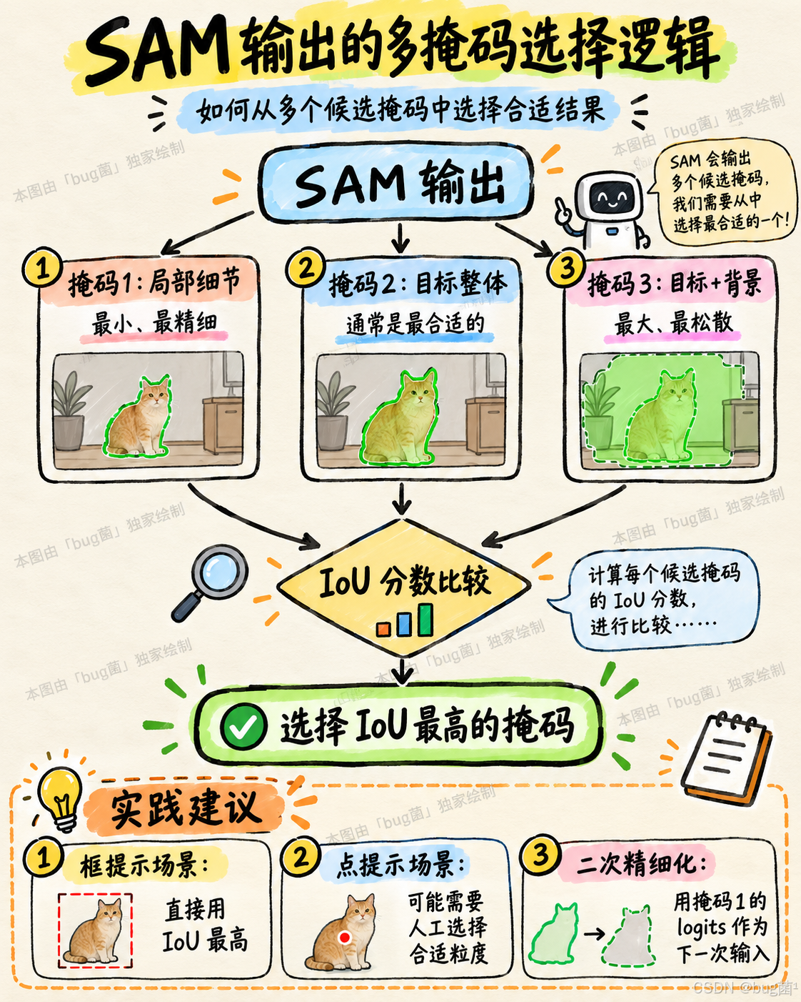
在全自动流水线中,直接选 IoU 分数最高的掩码是最可靠的策略。只有在需要人工审核或精细控制的场景下,才需要考虑三个候选掩码的差异。
八、标注质量评估:如何知道自动标注做得好不好
自动标注产出了一批标注文件,但这些标注是否可信?是否可以直接用于训练?这是一个非常重要但经常被忽视的问题。
8.1 量化评估方法
如果你有少量人工标注的"黄金数据"(Ground Truth),可以用它来评估自动标注的质量:
# ============================================================
# 标注质量评估工具
# 功能:计算自动标注与人工标注之间的 IoU 对比
# ============================================================

import numpy as np
import json
from pathlib import Path
from typing import List, Dict, Tuple

def compute_mask_iou(mask1: np.ndarray, mask2: np.ndarray) -> float:
    """
    计算两个二值掩码之间的 IoU(Intersection over Union)

    IoU = 交集面积 / 并集面积

    Args:
        mask1: 第一个掩码(bool 数组)
        mask2: 第二个掩码(bool 数组)

    Returns:
        IoU 值,范围 [0, 1]
    """
    intersection = np.logical_and(mask1, mask2).sum()
    union = np.logical_or(mask1, mask2).sum()

    if union == 0:
        return 0.0

    return float(intersection) / float(union)


def compute_bbox_iou(
    bbox1: List[float],  # [x1, y1, x2, y2]
    bbox2: List[float]   # [x1, y1, x2, y2]
) -> float:
    """
    计算两个边界框的 IoU

    Args:
        bbox1, bbox2: [x1, y1, x2, y2] 格式的边界框

    Returns:
        IoU 值,范围 [0, 1]
    """
    x1 = max(bbox1[0], bbox2[0])
    y1 = max(bbox1[1], bbox2[1])
    x2 = min(bbox1[2], bbox2[2])
    y2 = min(bbox1[3], bbox2[3])

    intersection = max(0, x2 - x1) * max(0, y2 - y1)

    area1 = (bbox1[2] - bbox1[0]) * (bbox1[3] - bbox1[1])
    area2 = (bbox2[2] - bbox2[0]) * (bbox2[3] - bbox2[1])

    union = area1 + area2 - intersection

    if union <= 0:
        return 0.0

    return intersection / union


def evaluate_annotation_quality(
    auto_label_dir: str,
    gt_label_dir: str,
    image_dir: str,
    iou_threshold: float = 0.5
) -> Dict:
    """
    对比自动标注与人工标注,计算质量指标

    这个函数假设两个目录中有相同文件名的 .txt 标注文件(YOLO 检测格式),
    计算在给定 IoU 阈值下的 Precision、Recall、F1 等指标。

    Args:
        auto_label_dir: 自动标注目录
        gt_label_dir: 人工标注(Ground Truth)目录
        image_dir: 对应图像目录(用于获取图像尺寸)
        iou_threshold: 判定为正确匹配的 IoU 阈值

    Returns:
        评估指标字典
    """
    import cv2

    auto_label_dir = Path(auto_label_dir)
    gt_label_dir = Path(gt_label_dir)
    image_dir = Path(image_dir)

    # 查找共同的文件
    auto_files = {p.stem: p for p in auto_label_dir.glob("*.txt")}
    gt_files = {p.stem: p for p in gt_label_dir.glob("*.txt")}
    common_stems = set(auto_files.keys()) & set(gt_files.keys())

    if not common_stems:
        print("警告:没有找到共同的标注文件!")
        return {}

    print(f"评估 {len(common_stems)} 张图像的标注质量...")

    total_tp = 0  # True Positive: 正确标注的目标数
    total_fp = 0  # False Positive: 自动标注中多出的目标数
    total_fn = 0  # False Negative: 自动标注中漏掉的目标数

    iou_scores = []  # 所有匹配对的 IoU 分数

    def read_yolo_labels(txt_path, img_w, img_h):
        """读取 YOLO 检测格式的标注文件,返回绝对坐标的 bbox 列表"""
        bboxes = []
        with open(txt_path, "r") as f:
            for line in f.read().strip().split("\n"):
                if not line:
                    continue
                parts = line.split()
                if len(parts) < 5:
                    continue
                class_id = int(parts[0])
                cx, cy, w, h = map(float, parts[1:5])
                x1 = (cx - w/2) * img_w
                y1 = (cy - h/2) * img_h
                x2 = (cx + w/2) * img_w
                y2 = (cy + h/2) * img_h
                bboxes.append({"class_id": class_id, "bbox": [x1, y1, x2, y2]})
        return bboxes

    for stem in common_stems:
        # 获取图像尺寸
        img_path = None
        for ext in [".jpg", ".jpeg", ".png", ".bmp"]:
            p = image_dir / (stem + ext)
            if p.exists():
                img_path = p
                break

        if img_path is None:
            continue

        img = cv2.imread(str(img_path))
        if img is None:
            continue
        img_h, img_w = img.shape[:2]

        # 读取标注
        auto_bboxes = read_yolo_labels(auto_files[stem], img_w, img_h)
        gt_bboxes = read_yolo_labels(gt_files[stem], img_w, img_h)

        # 匹配自动标注和 GT(贪心匹配,按 IoU 从高到低)
        matched_auto = set()
        matched_gt = set()

        # 计算所有 auto-gt 对的 IoU
        iou_matrix = np.zeros((len(auto_bboxes), len(gt_bboxes)))
        for i, auto_det in enumerate(auto_bboxes):
            for j, gt_det in enumerate(gt_bboxes):
                if auto_det["class_id"] == gt_det["class_id"]:
                    iou = compute_bbox_iou(auto_det["bbox"], gt_det["bbox"])
                    iou_matrix[i, j] = iou

        # 贪心匹配
        while True:
            if iou_matrix.size == 0:
                break
            max_iou = iou_matrix.max()
            if max_iou < iou_threshold:
                break
            i, j = np.unravel_index(iou_matrix.argmax(), iou_matrix.shape)
            matched_auto.add(i)
            matched_gt.add(j)
            iou_scores.append(max_iou)
            iou_matrix[i, :] = -1  # 标记已匹配
            iou_matrix[:, j] = -1

        tp = len(matched_auto)
        fp = len(auto_bboxes) - tp
        fn = len(gt_bboxes) - len(matched_gt)

        total_tp += tp
        total_fp += fp
        total_fn += fn

    # 计算 Precision、Recall、F1
    precision = total_tp / (total_tp + total_fp) if (total_tp + total_fp) > 0 else 0
    recall = total_tp / (total_tp + total_fn) if (total_tp + total_fn) > 0 else 0
    f1 = 2 * precision * recall / (precision + recall) if (precision + recall) > 0 else 0

    avg_iou = np.mean(iou_scores) if iou_scores else 0

    results = {
        "num_evaluated_images": len(common_stems),
        "true_positives": total_tp,
        "false_positives": total_fp,
        "false_negatives": total_fn,
        "precision": precision,
        "recall": recall,
        "f1_score": f1,
        "average_iou": avg_iou,
        "iou_threshold": iou_threshold
    }

    print("\n标注质量评估结果:")
    print(f"  Precision(精确率): {precision:.4f}")
    print(f"  Recall(召回率):   {recall:.4f}")
    print(f"  F1 Score:            {f1:.4f}")
    print(f"  平均 IoU:            {avg_iou:.4f}")
    print(f"  漏标(FN):          {total_fn}")
    print(f"  误标(FP):          {total_fp}")

    return results
8.2 人工抽检策略
即使量化指标看起来不错,人工抽检也是必要的。我在项目中通常遵循以下抽检策略:
按置信度分层抽检:把检测结果按照 YOLOv10 置信度分成高(>0.7)、中(0.45-0.7)、低(<0.45)三档,在每档中各抽取 30-50 张图进行人工核查。通常低置信度档的误标率会明显更高,这个结论可以帮助你确定合适的置信度阈值。
按类别抽检:对每个类别单独做抽检,因为不同类别的自动标注质量差异可能很大。外形相似的类别(比如"猫"和"狗"从框的形状看差不多)误标率可能更高。
问题图像优先:挑选那些目标密集、遮挡严重、光线不佳的图像重点核查,这些场景下自动标注更容易出错。
九、流水线优化:让它跑得更快
标注 10 万张图,哪怕每张 1 秒,也需要 27 小时。优化速度是工程上不可绕过的话题。
9.1 批量推理优化
# ============================================================
# 批量推理优化:同时处理多张图像
# ============================================================

from ultralytics import YOLO
import torch
import numpy as np
import cv2
from typing import List

def batch_yolo_inference(
    model: YOLO,
    images: List[np.ndarray],
    batch_size: int = 8,
    conf: float = 0.45
) -> List[List[dict]]:
    """
    对图像列表进行批量 YOLOv10 推理

    批量推理的优势:
    - GPU 利用率从单张推理的 30-50% 提升到 80-90%
    - 吞吐量(throughput)显著提升
    - 适合在有 GPU 的服务器上大规模标注

    Args:
        model: YOLOv10 模型实例
        images: 图像列表(BGR 格式)
        batch_size: 批次大小(根据 GPU 显存调整)
        conf: 置信度阈值

    Returns:
        每张图像的检测结果列表(与输入 images 一一对应)
    """
    all_results = []

    # 按 batch_size 切分,逐批处理
    for i in range(0, len(images), batch_size):
        batch = images[i:i + batch_size]

        # ultralytics 支持直接传入图像列表进行批量推理
        batch_results = model(
            batch,
            conf=conf,
            verbose=False
        )

        # 解析每张图的结果
        for result in batch_results:
            image_detections = []

            if result.boxes is not None:
                for box in result.boxes:
                    img_h, img_w = result.orig_shape
                    x1, y1, x2, y2 = box.xyxy[0].tolist()
                    x1, y1, x2, y2 = int(x1), int(y1), int(x2), int(y2)
                    w = x2 - x1
                    h = y2 - y1

                    image_detections.append({
                        "bbox_xyxy": [x1, y1, x2, y2],
                        "bbox_normalized": [
                            (x1 + w/2)/img_w, (y1 + h/2)/img_h,
                            w/img_w, h/img_h
                        ],
                        "class_id": int(box.cls.item()),
                        "confidence": float(box.conf.item())
                    })

            all_results.append(image_detections)

    return all_results


def estimate_processing_time(
    num_images: int,
    has_gpu: bool = True,
    sam_model: str = "sam2_b"
) -> dict:
    """
    估算处理时间(基于经验值)

    这些数值基于典型硬件(RTX 3090)的实测结果,
    实际时间因硬件和图像内容而异。

    Args:
        num_images: 图像总数
        has_gpu: 是否有 GPU
        sam_model: SAM 模型规格

    Returns:
        时间估算字典
    """
    # 单张图像处理时间(秒)的经验估计
    # 基于 RTX 3090, 640x480 图像, 平均 5 个目标/图
    time_per_image_estimates = {
        ("gpu", "sam_b"):  0.15,  # YOLOv10: ~30ms, SAM: ~80ms, 后处理: ~40ms
        ("gpu", "sam_l"):  0.25,
        ("gpu", "sam_h"):  0.50,
        ("gpu", "sam2_b"): 0.12,  # SAM2 比 SAM 快约 20%
        ("gpu", "sam2_l"): 0.20,
        ("cpu", "sam_b"):  3.50,  # CPU 慢约 20-30 倍
        ("cpu", "sam2_b"): 2.80,
    }

    device = "gpu" if has_gpu else "cpu"
    key = (device, sam_model)

    time_per_image = time_per_image_estimates.get(key, 0.3)
    total_seconds = num_images * time_per_image

    return {
        "num_images": num_images,
        "device": device,
        "sam_model": sam_model,
        "estimated_seconds": total_seconds,
        "estimated_minutes": total_seconds / 60,
        "estimated_hours": total_seconds / 3600,
        "throughput_per_hour": int(3600 / time_per_image)
    }


# 时间估算示例
est = estimate_processing_time(10000, has_gpu=True, sam_model="sam2_b")
print(f"\n时间估算({est['num_images']} 张图,{est['device'].upper()},{est['sam_model']}):")
print(f"  预估总时间: {est['estimated_hours']:.1f} 小时")
print(f"  处理吞吐量: {est['throughput_per_hour']} 张/小时")
9.2 多进程并行优化
# ============================================================
# 多进程并行优化:充分利用多 GPU 或多 CPU 核心
# ============================================================

import multiprocessing as mp
from pathlib import Path
import os

def worker_process(
    worker_id: int,
    image_list: list,
    output_dir: str,
    yolo_model: str,
    sam_model: str,
    conf_threshold: float,
    device_id: int
):
    """
    工作进程函数

    在多 GPU 场景下,每个 GPU 运行一个独立的进程,
    各自负责处理一部分图像,互不干扰。

    Args:
        worker_id: 进程编号
        image_list: 该进程负责的图像列表
        output_dir: 输出目录
        yolo_model: YOLOv10 模型路径
        sam_model: SAM 模型名称
        conf_threshold: 置信度阈值
        device_id: GPU 设备编号
    """
    import torch

    print(f"[Worker {worker_id}] 启动,负责 {len(image_list)} 张图像")
    print(f"[Worker {worker_id}] 使用 GPU: {device_id}")

    # 在子进程中初始化模型(避免主进程的模型被 fork 后状态不一致)
    device = f"cuda:{device_id}" if torch.cuda.is_available() else "cpu"

    pipeline = SAMYOLOAnnotationPipeline(
        yolo_model_path=yolo_model,
        sam_model_name=sam_model,
        conf_threshold=conf_threshold,
        device=device
    )

    label_dir = os.path.join(output_dir, "labels")

    for i, image_path in enumerate(image_list):
        try:
            pipeline.process_single_image(
                image_path,
                label_dir,
                visualize=False
            )

            if (i + 1) % 100 == 0:
                print(f"[Worker {worker_id}] 已处理 {i+1}/{len(image_list)}")

        except Exception as e:
            print(f"[Worker {worker_id}] 处理失败: {image_path}: {e}")

    print(f"[Worker {worker_id}] 完成!")


def run_parallel_annotation(
    image_dir: str,
    output_dir: str,
    yolo_model: str = "yolov10s.pt",
    sam_model: str = "sam2_b.pt",
    conf_threshold: float = 0.45,
    num_gpus: int = None
):
    """
    多 GPU 并行自动标注

    Args:
        image_dir: 图像目录
        output_dir: 输出目录
        yolo_model: YOLOv10 模型
        sam_model: SAM 模型
        conf_threshold: 置信度阈值
        num_gpus: 使用的 GPU 数量(None 则自动检测)
    """
    import torch

    # 检测可用 GPU 数量
    if num_gpus is None:
        num_gpus = torch.cuda.device_count() if torch.cuda.is_available() else 1

    print(f"多 GPU 并行标注")
    print(f"  使用 GPU 数量: {num_gpus}")

    # 收集所有图像
    image_dir = Path(image_dir)
    all_images = []
    for ext in [".jpg", ".jpeg", ".png", ".bmp"]:
        all_images.extend([str(p) for p in image_dir.glob(f"*{ext}")])

    print(f"  图像总数: {len(all_images)}")

    # 将图像列表均匀分配给各个 GPU
    chunks = [[] for _ in range(num_gpus)]
    for i, img in enumerate(all_images):
        chunks[i % num_gpus].append(img)

    # 启动多进程
    processes = []
    for worker_id, (chunk, gpu_id) in enumerate(zip(chunks, range(num_gpus))):
        p = mp.Process(
            target=worker_process,
            args=(worker_id, chunk, output_dir, yolo_model, sam_model,
                  conf_threshold, gpu_id)
        )
        p.start()
        processes.append(p)

    # 等待所有进程完成
    for p in processes:
        p.join()

    print("\n所有工作进程完成!")
十、从框到 Mask 到标签:完整数据流可视化
让我们用一张综合性的流程图把本节所有内容串联起来:
相关示意图绘制如下,仅供参考:
十一、常见问题与解决方案
在实际使用 SAM + YOLOv10 联合标注的过程中,我踩过不少坑,这里整理成 FAQ,希望能帮你省去不必要的弯路。
Q1:SAM 分割出来的掩码和目标框对不上,边界明显偏移?
通常有两个原因:一是坐标系不一致(OpenCV 是 BGR,SAM 原版需要 RGB),一定要注意颜色通道转换;二是图像在送入 SAM 之前做了缩放,但提供给 SAM 的框坐标是原始图像的坐标,要保持一致。
Q2:处理速度非常慢,大概每张图需要 3-5 秒?
如果你用的是 CPU,这是正常的——SAM 的 ViT 编码器在 CPU 上非常慢。解决方案是换 GPU,或者退而求其次,使用 sam_b(ViT-B)代替 sam_h,速度差距接近 5 倍。另外,确认你的批量推理是否真正生效,很多人以为自己在批量推理,其实还是在逐张处理。
Q3:自动标注的掩码总是比目标大一圈,有"膨胀"现象?
这通常是因为 YOLOv10 的检测框本身就不够贴合目标,有一定的"留白",SAM 在这个放大的区域内分割,边界自然会宽松。尝试把 YOLOv10 的 NMS IoU 阈值从 0.45 调到 0.35,让框更紧,SAM 的结果也会随之改善。
Q4:某些类别(比如细长的目标、透明物体)的掩码效果很差?
细长目标(电线、铁轨)和透明物体(玻璃杯、水)是 SAM 的弱项,原因在于 SA-1B 数据集虽然大,但这类样本本身就难以收集和标注。对于这类目标,建议降低对 SAM 的期望,改用检测框标注而非分割标注,或者接受更多人工修正的工作量。
Q5:生成的 .txt 标注文件打开 YOLO 训练,报 “invalid label” 错误?
这通常是多边形顶点坐标超出了 [0, 1] 范围。检查你的归一化代码,确保所有坐标都被 max(0, min(1, x)) 截断。边界处的掩码可能会有轮廓点落在图像外,需要做边界限制。
十二、进阶应用:半自动标注工作流
全自动标注虽然高效,但在精度要求极高的场景(医疗、安防、工业质检)下,往往需要人工参与修正。半自动标注工作流是一个更实用的折中方案:AI 完成 80% 的粗标注工作,人工只需要审核和修正剩余 20% 的问题标注。
相关示意图绘制如下,仅供参考:
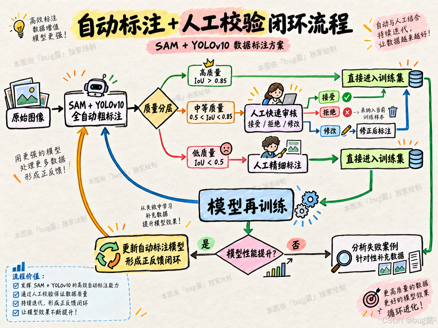
这个工作流的精髓在于主动学习的思想:AI 对自己不确定的样本标记"低质量",人工只需要专注处理这些难例,而不是对所有图像一视同仁。随着人工修正的样本不断加入训练集,模型越来越强,自动标注的质量也越来越高,最终形成正反馈闭环。
这个思路也直接引出了我们下一章要讲的主题——伪标签训练和主动学习,后面的章节会深入展开。
📌 本节总结
走完这一节,你应该对 SAM + YOLOv10 联合自动标注有了完整的认识。我们从原理出发,理解了 SAM 为什么能凭借一个检测框就精确分割目标;从工程角度,我们搭建了一个包含检测、分割、格式转换、质量评估的完整流水线;从实践角度,我们讨论了常见的坑和优化手段。
几个需要重点记住的关键结论:
第一,YOLOv10 框 = SAM 提示,这是两个模型协同的核心接口,框的质量直接决定分割质量。
第二,图像编码只做一次,SAM 的 set_image() / 图像缓存机制是大规模标注场景中最关键的性能优化。
第三,置信度阈值在标注场景要比推理场景设高,宁可少标,不能错标,标注噪声比标注缺失危害更大。
第四,掩码多边形简化是必要的,Douglas-Peucker 算法能在几乎不损失精度的前提下,把几百个轮廓点压缩到十几个,显著减小标注文件体积。
第五,全自动标注要搭配质量评估,不管是量化指标对比还是人工抽检,都是保证训练数据质量的必要环节。
🔮 下期预告:GroundingDINO + SAM + YOLOv10 零样本标注流水线
下一节,我们要在本节的基础上更进一步,引入 GroundingDINO 这个重磅工具。
如果说本节的 SAM + YOLOv10 方案需要"先有 YOLOv10 模型"才能提供检测框,那么下一节要解决的问题是:如果连检测模型都没有怎么办?
GroundingDINO 是一个语言引导的开放集目标检测模型,你可以用自然语言描述你想检测的对象——“一个带红色标签的瓶子”、“破损的工件表面”——它就能在图像中定位这些目标,完全不需要预先训练针对这些类别的检测器。
下一节的流水线将是:
- GroundingDINO:用文字描述定位目标,生成边界框(零样本检测)
- SAM:精细分割(像素级掩码)
- YOLOv10:利用这批自动标注的数据训练定制检测器(冷启动)
这三者的组合,构成了一个"从零到有"的完整目标检测冷启动方案——你只需要一些无标注图像和几句文字描述,就能端到端地构建一个针对特定场景的 YOLOv10 检测器。
这是生成式 AI 赋能 YOLO 最令人兴奋的应用场景之一,下节见。
作者注:本节所有代码已尽量设计为可直接运行的形式,但实际执行时需要根据你的具体环境调整路径、模型选择和硬件配置。SAM 和 YOLOv10 的官方文档是最权威的参考来源,遇到接口变化时以官方文档为准。如果你在实际操作中遇到了问题,或者有更好的优化思路,欢迎在评论区交流。
📌 附录
相关参考资料
- YOLOv10 官方论文:YOLOv10: Real-Time End-to-End Object Detection,Wang et al., 2024,arXiv: 2405.14458
- YOLOv10 核心机制:Consistent Dual Assignments(一致性双重标签分配)
- YOLOv10 端到端检测机制:One-to-Many + One-to-One Dual Assignments
- YOLOv10 高效模型设计:Holistic Efficiency-Accuracy Driven Model Design
- YOLOv10 NMS-Free 推理:End-to-End Object Detection without NMS
- DFL 相关:Generalized Focal Loss: Learning Qualified and Distributed Bounding Boxes for Dense Object Detection
- COCO 数据集基准:https://cocodataset.org
- YOLOv10 官方仓库:https://github.com/THU-MIG/yolov10
- PyTorch 官方安装指南:https://pytorch.org/get-started/locally/
- NVIDIA CUDA Toolkit 归档:https://developer.nvidia.com/cuda-toolkit-archive
- Miniconda 下载:https://docs.conda.io/en/latest/miniconda.html
- 本节所有脚本代码:见文章各代码块,可直接复制使用
COCO:
| Model | Test Size | AP^val | Params | FLOPs | Latency |
|---|---|---|---|---|---|
| YOLOv10-N | 640 | 38.5% | 2.3M | 6.7G | 1.84 ms |
| YOLOv10-S | 640 | 46.3% | 7.2M | 21.6G | 2.49 ms |
| YOLOv10-M | 640 | 51.1% | 15.4M | 59.1G | 4.74 ms |
| YOLOv10-B | 640 | 52.5% | 19.1M | 92.0G | 5.74 ms |
| YOLOv10-L | 640 | 53.2% | 24.4M | 120.3G | 7.28 ms |
| YOLOv10-X | 640 | 54.4% | 29.5M | 160.4G | 10.70 ms |
希望本文围绕 YOLOv10 的实战讲解,能够在以下几个维度上切实帮助到你:
- 🎯 模型精度提升:结合 YOLOv10 的一致性双重标签分配、端到端检测机制与整体效率-精度设计思想,从网络结构、特征融合、检测头、标签分配、损失函数和数据增强等方向展开优化,通过工程实验进一步提升目标检测精度;
- 🚀 推理速度优化:结合 YOLOv10 的 NMS-Free 推理机制,以及模型轻量化、结构重参数化、剪枝、量化、知识蒸馏与部署加速策略,帮助模型在真实业务场景中运行得更快、更稳定;
- 🧩 工程落地实践:覆盖数据准备、环境配置、模型训练、效果评估、问题排查、模型导出与部署推理等完整链路,提供可直接复用或稍加修改即可迁移的工程级方案;
- 🧠 核心机制理解:深入分析 YOLOv10 中 One-to-Many 与 One-to-One 双标签分配机制、一致性匹配度量、端到端检测以及高效网络设计 的设计逻辑,帮助你理解模型性能提升背后的原因,而不是停留在简单调用层面;
- 🔬 改进方案验证:通过消融实验、指标对比与可视化分析,评估不同改进模块对 Precision、Recall、mAP、FPS、Latency、参数量和 FLOPs 的实际影响。
PS:如果你按照文中步骤对 YOLOv10 进行优化后仍然遇到问题,请不必焦虑或灰心。
YOLOv10 是一个涉及网络结构、特征提取、标签分配、梯度优化、端到端预测与部署环境的复杂目标检测框架,最终表现会受到 硬件环境、数据集质量、任务定义、类别分布、训练配置、代码版本与部署平台 等多重因素的共同影响。
这是目标检测项目中十分常见的客观现象,并不意味着某个改进模块一定无效。
如果你在实践过程中遇到以下问题:
- 🐛 模块替换后出现新的报错或 Bug;
- 📉 Precision、Recall 或 mAP 难以继续提升;
- 📈 训练损失异常、梯度不稳定或模型难以收敛;
- 🎯 One-to-One / One-to-Many 分支训练效果异常;
- ⏱️ 推理速度、Latency、显存占用或部署性能不达预期;
- 🔄 修改网络结构后出现维度、通道数或特征层不匹配;
- ⚙️ 修改检测头后端到端预测分支出现兼容性问题;
- 📦 模型导出 ONNX、TensorRT、OpenVINO 等格式时失败;
欢迎将 完整报错信息 + 环境版本 + 关键配置截图 + 网络配置文件 + 核心代码片段 粘贴至评论区,我们可以一起分析问题根因,并探讨更加可行的解决方案。
如果你已经摸索出更优的训练参数、网络结构、标签分配策略、模块组合或部署优化思路,也非常欢迎在评论区分享。
你的每一条实战经验,都可能成为其他开发者解决问题、减少试错成本的关键线索。
部分章节还会结合国内外前沿论文与 AIGC 大模型技术,对 YOLOv10 的主流改进方案进行重构与再设计,使内容更加贴近工业检测、智慧交通、游戏分析、行为识别、遥感影像、无人机视觉与边缘设备部署等真实应用场景。
🧧🧧 文末福利,等你来拿!🧧🧧
📌 文中所涉及的技术内容,大多来源于本人在 YOLOv10 项目中的一线实践积累,部分案例参考了开源项目、公开论文、技术社区资料与读者反馈。
如有版权相关问题,欢迎第一时间联系,我将尽快核实并进行修改或下线处理。
部分问题分析思路与排查路径参考了技术社区及 AI 问答平台,在此一并致谢 🙏
最后想说的是:
YOLOv10 的优化本质上是一个高度依赖任务、数据和部署环境的系统工程问题,不存在“一招通杀”的银弹方案。
一致性双重标签分配、One-to-Many / One-to-One 检测策略、注意力机制、轻量化卷积、改进检测头、IoU 损失函数、特征融合模块和数据增强策略,都有其适用条件。
某个模块在公开数据集上取得提升,并不意味着它能够在所有自定义数据集、硬件平台和业务场景中获得同样收益。
尤其对于 YOLOv10 而言,在进行结构改进时还需要额外关注 端到端检测分支、标签分配一致性以及 NMS-Free 推理链路。某些直接从 YOLOv8、YOLOv9、YOLOv11 等模型迁移过来的模块,如果没有处理好检测头与训练分支之间的适配关系,也可能出现精度下降、训练不稳定或推理逻辑异常等问题。
真正有效的优化路径,永远源于:
- 对业务目标与评价指标的准确理解;
- 对数据质量和类别分布的持续分析;
- 对模型瓶颈的定位与针对性改进;
- 对 One-to-Many 与 One-to-One 分支机制的正确理解;
- 对实验变量的严格控制;
- 对精度、速度、Latency、参数量和部署成本的综合权衡;
- 以及一轮又一轮可复现的对比实验。
如果你已经在自己的项目中探索出了更加高效、稳定的 YOLOv10 优化路径,非常鼓励你:
- 💬 在评论区简要分享核心思路与实验结论;
- 📊 分享不同模块的消融实验结果;
- 📝 将完整过程整理成教程、博客或系列文章;
- 🔧 提交可复现的配置文件、代码或工程实践经验。
你的经验,或许正是别人卡关已久所缺少的最后一块拼图。
✅ 本期关于 YOLOv10 优化与实战应用 的内容就先聊到这里。
如果你想进一步深入:
- 🔍 系统理解 Consistent Dual Assignments 与 YOLOv10 的整体网络结构;
- 🎯 深入理解 One-to-Many 与 One-to-One 双标签分配机制;
- 🚀 掌握 YOLOv10 无 NMS 端到端目标检测的实现原理;
- 🧱 学习主干网络、颈部网络、检测头与特征融合模块的改进方法;
- 📉 掌握损失函数、匹配度量、样本分配与训练策略的优化技巧;
- ⚡ 对比不同场景下的模型轻量化与部署加速方案;
- 🧪 建立规范的消融实验、指标对比与模型评估流程;
- 🧠 系统构建一套属于自己的 YOLOv10 调优方法论;
欢迎继续关注专栏:《YOLOv10实战:从入门到深度优化》
期待这些内容能够在你的项目中真正落地见效,帮助你 少踩坑、多提效、快验证、稳部署,我们下期见。
✨ 当然,如果 YOLOv10 专栏已经无法满足你,也可以继续关注:
更多新版本、新模块与新论文的工程复现内容,也会持续更新。
✍️ 码字不易,如果这篇文章对你有所启发或帮助,欢迎给我来个 一键三连:关注 + 点赞 + 收藏。
你的支持,是我持续输出高质量 YOLOv10 技术内容与工程实战案例最直接的动力来源。
同时诚挚推荐关注我的技术号: 「猿圈奇妙屋」
在这里,你可以:
- 📡 第一时间获取 YOLOv10、目标检测、多目标追踪与多任务学习等方向的进阶内容;
- 🛠️ 获取视觉算法、深度学习与模型部署的最新优化方案和工程实战经验;
- 📚 学习 PyTorch、OpenCV、ONNX、TensorRT 等相关技术;
- 🎁 获取 BAT 大厂面经、技术书籍 PDF、工程模板与常用工具清单等实用资源。
期待在更多维度上与你一起进步、共同成长。
👨💻 About Me · 关于作者
我是专注于 计算机视觉、图像识别、目标检测与深度学习工程落地 的讲师和技术博主,笔名 bug菌:
- 活跃于 CSDN|稀土掘金|InfoQ|51CTO|华为云开发者社区|阿里云开发者社区|腾讯云开发者社区|开源中国|博客园|墨天轮 等多个技术社区;
- CSDN 博客之星 Top 30、华为云多年度十佳博主及卓越贡献奖获得者、掘金多年度人气作者 Top 40;
- CSDN、掘金、InfoQ、51CTO 等平台签约作者及优质创作者;
- 全网粉丝累计 30w+。
更多高质量技术内容与成长资料,可查看合集入口:
👉 点击查看 👈️
硬核技术号 「猿圈奇妙屋」 期待你的加入,一起进阶、一起打怪升级。

- End -

有“AI”的1024 = 2048,欢迎大家加入2048 AI社区
更多推荐

 1
1 0
0- 0


 已为社区贡献63条内容

所有评论(0)