第089篇:海洋平台水动力学
本教程介绍海洋平台的水动力学仿真方法。通过建立波浪-结构相互作用的数学模型,实现海洋平台的运动响应和载荷预测。教程涵盖波浪理论、Morison方程、绕射理论、平台运动响应以及系泊系统分析等内容。海洋平台,波浪理论,Morison方程,绕射理论,系泊系统线性波浪理论(Airy波):波面方程:η=Acos(kx−ωt)\eta = A \cos(kx - \omega t)η=Acos(kx−ωt)
第089篇:海洋平台水动力学
摘要
本教程介绍海洋平台的水动力学仿真方法。通过建立波浪-结构相互作用的数学模型,实现海洋平台的运动响应和载荷预测。教程涵盖波浪理论、Morison方程、绕射理论、平台运动响应以及系泊系统分析等内容。
关键词
海洋平台,波浪理论,Morison方程,绕射理论,系泊系统
1. 理论基础
1.1 波浪理论
线性波浪理论(Airy波):
波面方程:
η=Acos(kx−ωt)\eta = A \cos(kx - \omega t)η=Acos(kx−ωt)
色散关系:
ω2=gktanh(kd)\omega^2 = gk \tanh(kd)ω2=gktanh(kd)
其中:
- AAA 为波幅
- kkk 为波数
- ω\omegaω 为角频率
- ddd 为水深
水质点速度:
u=gAkωcoshk(z+d)coshkdcos(kx−ωt)u = \frac{gAk}{\omega} \frac{\cosh k(z+d)}{\cosh kd} \cos(kx - \omega t)u=ωgAkcoshkdcoshk(z+d)cos(kx−ωt)
w=gAkωsinhk(z+d)coshkdsin(kx−ωt)w = \frac{gAk}{\omega} \frac{\sinh k(z+d)}{\cosh kd} \sin(kx - \omega t)w=ωgAkcoshkdsinhk(z+d)sin(kx−ωt)
1.2 Morison方程
对于小尺度结构(直径与波长比 < 0.2),采用Morison方程计算波浪力:
F=FD+FI=12ρCDDu∣u∣+ρCMπD24u˙F = F_D + F_I = \frac{1}{2} \rho C_D D u|u| + \rho C_M \frac{\pi D^2}{4} \dot{u}F=FD+FI=21ρCDDu∣u∣+ρCM4πD2u˙
其中:
- CDC_DCD 为阻力系数(通常1.0-1.2)
- CMC_MCM 为惯性系数(通常1.5-2.0)
- DDD 为结构直径
1.3 绕射理论
对于大尺度结构,需要考虑波浪绕射效应。采用势流理论,速度势满足Laplace方程:
∇2ϕ=0\nabla^2 \phi = 0∇2ϕ=0
边界条件:
- 自由表面条件
- 底部边界条件
- 结构物边界条件(法向速度连续)
- 辐射条件
1.4 平台运动方程
六自由度运动方程:
(M+A)ξ¨+Bξ˙+Cξ=Fwave+Fmooring(M + A)\ddot{\xi} + B\dot{\xi} + C\xi = F_{wave} + F_{mooring}(M+A)ξ¨+Bξ˙+Cξ=Fwave+Fmooring
其中:
- MMM 为质量矩阵
- AAA 为附加质量矩阵
- BBB 为阻尼矩阵
- CCC 为恢复力矩阵
- ξ\xiξ 为位移向量
2. Python实现
import matplotlib
matplotlib.use('Agg')
import numpy as np
import matplotlib.pyplot as plt
from matplotlib.patches import Rectangle, Circle, FancyBboxPatch, Polygon, FancyArrowPatch
import warnings
warnings.filterwarnings('ignore')
import os
# 创建输出目录
output_dir = r'd:\文档\流体动力学\主题089'
os.makedirs(output_dir, exist_ok=True)
print("=" * 60)
print("海洋平台水动力学仿真")
print("=" * 60)
class WaveTheory:
"""波浪理论"""
def __init__(self, H=5, T=10, d=50):
self.H = H # 波高 (m)
self.T = T # 周期 (s)
self.d = d # 水深 (m)
self.g = 9.81
# 计算波数和频率
self.omega = 2 * np.pi / T
self.k = self.solve_dispersion()
self.L = 2 * np.pi / self.k # 波长
self.A = H / 2 # 波幅
def solve_dispersion(self):
"""求解色散方程"""
# 迭代求解 k
k = 0.01
for _ in range(100):
k_new = self.omega**2 / (self.g * np.tanh(k * self.d))
if abs(k_new - k) < 1e-6:
break
k = 0.5 * k + 0.5 * k_new
return k
def elevation(self, x, t):
"""波面高度"""
return self.A * np.cos(self.k * x - self.omega * t)
def velocity(self, x, z, t):
"""水质点速度"""
cosh_kd = np.cosh(self.k * (z + self.d))
sinh_kd = np.sinh(self.k * self.d)
u = self.g * self.k * self.A / self.omega * cosh_kd / np.cosh(self.k * self.d) * \
np.cos(self.k * x - self.omega * t)
w = self.g * self.k * self.A / self.omega * sinh_kd / np.cosh(self.k * self.d) * \
np.sin(self.k * x - self.omega * t)
return u, w
def acceleration(self, x, z, t):
"""水质点加速度"""
cosh_kd = np.cosh(self.k * (z + self.d))
sinh_kd = np.sinh(self.k * self.d)
du_dt = self.g * self.k * self.A * cosh_kd / np.cosh(self.k * self.d) * \
np.sin(self.k * x - self.omega * t)
dw_dt = -self.g * self.k * self.A * sinh_kd / np.cosh(self.k * self.d) * \
np.cos(self.k * x - self.omega * t)
return du_dt, dw_dt
class MorisonForce:
"""Morison方程计算波浪力"""
def __init__(self, D=2.0, C_D=1.2, C_M=2.0, rho=1025):
self.D = D # 直径
self.C_D = C_D # 阻力系数
self.C_M = C_M # 惯性系数
self.rho = rho # 海水密度
def calc_force(self, u, du_dt, dz):
"""计算单位长度波浪力"""
# 阻力
F_D = 0.5 * self.rho * self.C_D * self.D * u * abs(u)
# 惯性力
F_I = self.rho * self.C_M * np.pi * self.D**2 / 4 * du_dt
return F_D + F_I
class OffshorePlatform:
"""海洋平台模型"""
def __init__(self, mass=10000, draft=20, D_column=10, n_columns=4):
self.mass = mass # 质量 (kg)
self.draft = draft # 吃水深度 (m)
self.D_column = D_column # 立柱直径 (m)
self.n_columns = n_columns # 立柱数量
# 水动力参数
self.A33 = mass * 0.5 # 垂向附加质量
self.B33 = 50000 # 垂向阻尼
# 恢复力系数
rho = 1025
g = 9.81
A_waterplane = n_columns * np.pi * (D_column/2)**2
self.C33 = rho * g * A_waterplane
def heave_response(self, omega, F_wave):
"""计算垂荡响应"""
# 频域响应
A_total = self.mass + self.A33
denominator = np.sqrt((self.C33 - A_total * omega**2)**2 + (self.B33 * omega)**2)
amplitude = abs(F_wave) / denominator
phase = np.arctan2(self.B33 * omega, self.C33 - A_total * omega**2)
return amplitude, phase
def time_domain_response(self, t, wave_force):
"""时域运动响应"""
# 简化的单自由度运动方程求解
dt = t[1] - t[0]
z = np.zeros_like(t)
v = np.zeros_like(t)
a = np.zeros_like(t)
A_total = self.mass + self.A33
for i in range(1, len(t)):
# 加速度
a[i] = (wave_force[i] - self.B33 * v[i-1] - self.C33 * z[i-1]) / A_total
# 速度和位移(Newmark-beta方法简化)
v[i] = v[i-1] + a[i] * dt
z[i] = z[i-1] + v[i] * dt
return z, v, a
class MooringSystem:
"""系泊系统模型"""
def __init__(self, n_lines=8, L=500, w=500, EA=1e9, anchor_radius=300):
self.n_lines = n_lines # 系泊线数量
self.L = L # 系泊线长度 (m)
self.w = w # 单位长度重量 (N/m)
self.EA = EA # 轴向刚度 (N)
self.anchor_radius = anchor_radius # 锚点半径 (m)
def calc_restoring_force(self, x, y):
"""计算系泊恢复力"""
F_x = 0
F_y = 0
for i in range(self.n_lines):
angle = 2 * np.pi * i / self.n_lines
# 锚点位置
x_anchor = self.anchor_radius * np.cos(angle)
y_anchor = self.anchor_radius * np.sin(angle)
# 系泊线伸长
delta_L = np.sqrt((x_anchor - x)**2 + (y_anchor - y)**2) - self.anchor_radius
# 系泊力(简化线性模型)
if delta_L > 0:
T = self.EA * delta_L / self.L
F_x += T * (x_anchor - x) / np.sqrt((x_anchor - x)**2 + (y_anchor - y)**2)
F_y += T * (y_anchor - y) / np.sqrt((x_anchor - x)**2 + (y_anchor - y)**2)
return F_x, F_y
print("✓ 海洋平台水动力学模型定义完成")
# ============ 仿真1: 波浪场 ============
print("\n正在生成波浪场...")
wave = WaveTheory(H=5, T=10, d=50)
x = np.linspace(0, 200, 200)
t_snapshots = [0, 2.5, 5, 7.5]
fig, axes = plt.subplots(2, 2, figsize=(14, 11))
# 不同时间的波面形状
ax1 = axes[0, 0]
for t in t_snapshots:
eta = wave.elevation(x, t)
ax1.plot(x, eta, linewidth=2, label=f't = {t:.1f}s')
ax1.axhline(y=0, color='k', linestyle='--', alpha=0.3)
ax1.set_xlabel('x (m)', fontsize=11)
ax1.set_ylabel('Wave Elevation (m)', fontsize=11)
ax1.set_title('Wave Profiles at Different Times', fontsize=12, fontweight='bold')
ax1.legend(loc='upper right', fontsize=9)
ax1.grid(True, alpha=0.3)
ax1.set_xlim(0, 200)
# 水质点速度场
ax2 = axes[0, 1]
x_grid = np.linspace(0, 100, 20)
z_grid = np.linspace(-50, 0, 10)
X, Z = np.meshgrid(x_grid, z_grid)
t_plot = 0
U = np.zeros_like(X)
W = np.zeros_like(Z)
for i in range(len(z_grid)):
for j in range(len(x_grid)):
u, w = wave.velocity(x_grid[j], z_grid[i], t_plot)
U[i, j] = u
W[i, j] = w
ax2.quiver(X, Z, U, W, scale=50)
ax2.set_xlabel('x (m)', fontsize=11)
ax2.set_ylabel('z (m)', fontsize=11)
ax2.set_title('Water Particle Velocity Field', fontsize=12, fontweight='bold')
ax2.axhline(y=0, color='b', linewidth=2)
ax2.set_ylim(-50, 5)
# 波浪参数随波高变化
ax3 = axes[1, 0]
H_range = np.linspace(2, 10, 20)
L_range = []
for H in H_range:
wave_temp = WaveTheory(H=H, T=10, d=50)
L_range.append(wave_temp.L)
ax3.plot(H_range, L_range, 'b-', linewidth=2.5)
ax3.set_xlabel('Wave Height (m)', fontsize=11)
ax3.set_ylabel('Wavelength (m)', fontsize=11)
ax3.set_title('Wavelength vs Wave Height', fontsize=12, fontweight='bold')
ax3.grid(True, alpha=0.3)
# 色散关系
ax4 = axes[1, 1]
T_range = np.linspace(5, 20, 50)
k_values = []
for T in T_range:
wave_temp = WaveTheory(H=5, T=T, d=50)
k_values.append(wave_temp.k)
ax4.plot(T_range, k_values, 'r-', linewidth=2.5)
ax4.set_xlabel('Wave Period (s)', fontsize=11)
ax4.set_ylabel('Wave Number (rad/m)', fontsize=11)
ax4.set_title('Dispersion Relation', fontsize=12, fontweight='bold')
ax4.grid(True, alpha=0.3)
plt.tight_layout()
plt.savefig(f'{output_dir}/wave_field.png', dpi=150, bbox_inches='tight')
plt.close()
print("✓ 波浪场图已保存")
# ============ 仿真2: Morison力计算 ============
print("\n正在计算Morison力...")
morison = MorisonForce(D=2.0, C_D=1.2, C_M=2.0)
# 圆柱桩上的波浪力
t = np.linspace(0, 20, 500)
z_pile = np.linspace(-20, 0, 20) # 桩的垂直位置
x_pile = 0
# 计算波浪力
F_total = []
F_drag = []
F_inertia = []
for ti in t:
F_D_total = 0
F_I_total = 0
for zi in z_pile:
u, w = wave.velocity(x_pile, zi, ti)
du_dt, dw_dt = wave.acceleration(x_pile, zi, ti)
F_D = 0.5 * morison.rho * morison.C_D * morison.D * u * abs(u)
F_I = morison.rho * morison.C_M * np.pi * morison.D**2 / 4 * du_dt
F_D_total += F_D * (z_pile[1] - z_pile[0])
F_I_total += F_I * (z_pile[1] - z_pile[0])
F_drag.append(F_D_total)
F_inertia.append(F_I_total)
F_total.append(F_D_total + F_I_total)
fig, axes = plt.subplots(2, 2, figsize=(14, 11))
# 波浪力时程
ax1 = axes[0, 0]
ax1.plot(t, np.array(F_total)/1000, 'b-', linewidth=2, label='Total Force')
ax1.plot(t, np.array(F_drag)/1000, 'r--', linewidth=1.5, label='Drag Force')
ax1.plot(t, np.array(F_inertia)/1000, 'g--', linewidth=1.5, label='Inertia Force')
ax1.set_xlabel('Time (s)', fontsize=11)
ax1.set_ylabel('Force (kN)', fontsize=11)
ax1.set_title('Wave Force on Vertical Cylinder', fontsize=12, fontweight='bold')
ax1.legend(loc='upper right', fontsize=9)
ax1.grid(True, alpha=0.3)
# 阻力与惯性力比值
ax2 = axes[0, 1]
KC_numbers = np.linspace(0.1, 20, 50) # Keulegan-Carpenter数
F_ratio = []
for KC in KC_numbers:
# 简化的力比计算
ratio = (morison.C_D * KC) / (np.pi**2 * morison.C_M)
F_ratio.append(ratio)
ax2.semilogy(KC_numbers, F_ratio, 'b-', linewidth=2.5)
ax2.axhline(y=1, color='r', linestyle='--', alpha=0.7, label='Drag = Inertia')
ax2.set_xlabel('Keulegan-Carpenter Number', fontsize=11)
ax2.set_ylabel('Drag/Inertia Ratio', fontsize=11)
ax2.set_title('Drag vs Inertia Dominance', fontsize=12, fontweight='bold')
ax2.legend(loc='lower right', fontsize=9)
ax2.grid(True, alpha=0.3)
# 不同直径的波浪力
ax3 = axes[1, 0]
D_range = np.linspace(0.5, 5, 20)
F_max = []
for D in D_range:
morison_temp = MorisonForce(D=D, C_D=1.2, C_M=2.0)
F_temp = []
for ti in t[:100]:
F_D_total = 0
for zi in z_pile:
u, _ = wave.velocity(x_pile, zi, ti)
F_D = 0.5 * morison_temp.rho * morison_temp.C_D * morison_temp.D * u * abs(u)
F_D_total += F_D * (z_pile[1] - z_pile[0])
F_temp.append(F_D_total)
F_max.append(max(F_temp))
ax3.plot(D_range, np.array(F_max)/1000, 'b-', linewidth=2.5)
ax3.set_xlabel('Cylinder Diameter (m)', fontsize=11)
ax3.set_ylabel('Max Wave Force (kN)', fontsize=11)
ax3.set_title('Wave Force vs Cylinder Diameter', fontsize=12, fontweight='bold')
ax3.grid(True, alpha=0.3)
# 沿桩身的波浪力分布
ax4 = axes[1, 1]
t_plot = 0
F_distribution = []
for zi in z_pile:
u, _ = wave.velocity(x_pile, zi, t_plot)
du_dt, _ = wave.acceleration(x_pile, zi, t_plot)
F_D = 0.5 * morison.rho * morison.C_D * morison.D * u * abs(u)
F_I = morison.rho * morison.C_M * np.pi * morison.D**2 / 4 * du_dt
F_distribution.append((F_D + F_I) / 1000)
ax4.plot(F_distribution, z_pile, 'b-', linewidth=2.5)
ax4.axvline(x=0, color='k', linestyle='--', alpha=0.3)
ax4.set_xlabel('Force per Unit Length (kN/m)', fontsize=11)
ax4.set_ylabel('Depth (m)', fontsize=11)
ax4.set_title('Wave Force Distribution along Pile', fontsize=12, fontweight='bold')
ax4.grid(True, alpha=0.3)
plt.tight_layout()
plt.savefig(f'{output_dir}/morison_force.png', dpi=150, bbox_inches='tight')
plt.close()
print("✓ Morison力图已保存")
# ============ 仿真3: 平台运动响应 ============
print("\n正在计算平台运动响应...")
platform = OffshorePlatform(mass=10000, draft=20, D_column=10, n_columns=4)
# 不同波浪频率的响应
omega_range = np.linspace(0.1, 2.0, 50)
RAO = [] # 响应幅值算子
for omega in omega_range:
# 简化的波浪力计算
F_wave = 50000 * wave.A # 简化的波浪力幅值
amp, phase = platform.heave_response(omega, F_wave)
RAO.append(amp / wave.A)
fig, axes = plt.subplots(2, 2, figsize=(14, 11))
# RAO曲线
ax1 = axes[0, 0]
ax1.plot(omega_range, RAO, 'b-', linewidth=2.5)
ax1.axvline(x=np.sqrt(platform.C33 / (platform.mass + platform.A33)),
color='r', linestyle='--', alpha=0.7, label='Natural Frequency')
ax1.set_xlabel('Wave Frequency (rad/s)', fontsize=11)
ax1.set_ylabel('RAO (m/m)', fontsize=11)
ax1.set_title('Heave Response Amplitude Operator', fontsize=12, fontweight='bold')
ax1.legend(loc='upper right', fontsize=9)
ax1.grid(True, alpha=0.3)
# 时域响应
ax2 = axes[0, 1]
t_response = np.linspace(0, 60, 600)
# 生成波浪力时程
wave_force = 50000 * np.cos(wave.omega * t_response)
z, v, a = platform.time_domain_response(t_response, wave_force)
ax2.plot(t_response, z, 'b-', linewidth=2)
ax2.set_xlabel('Time (s)', fontsize=11)
ax2.set_ylabel('Heave Displacement (m)', fontsize=11)
ax2.set_title('Time Domain Heave Response', fontsize=12, fontweight='bold')
ax2.grid(True, alpha=0.3)
# 运动谱分析
ax3 = axes[1, 0]
# 简化的JONSWAP谱
f = np.linspace(0.05, 0.5, 100)
omega_spectrum = 2 * np.pi * f
fp = 2 * np.pi / wave.T # 峰值频率
alpha = 0.0081
gamma = 3.3
# PM谱
S_pm = alpha * 9.81**2 / (2 * np.pi)**4 / f**5 * np.exp(-1.25 * (fp / (2 * np.pi * f))**4)
ax3.semilogy(f, S_pm, 'b-', linewidth=2)
ax3.set_xlabel('Frequency (Hz)', fontsize=11)
ax3.set_ylabel('Spectral Density (m²/Hz)', fontsize=11)
ax3.set_title('Wave Spectrum (Pierson-Moskowitz)', fontsize=12, fontweight='bold')
ax3.grid(True, alpha=0.3)
# 响应谱
ax4 = axes[1, 1]
# 计算响应谱
S_response = []
for i, om in enumerate(omega_spectrum):
F_wave = 50000 * wave.A
amp, _ = platform.heave_response(om, F_wave)
S_response.append((amp / wave.A)**2 * S_pm[i])
ax4.semilogy(f, S_response, 'r-', linewidth=2)
ax4.set_xlabel('Frequency (Hz)', fontsize=11)
ax4.set_ylabel('Response Spectral Density (m²/Hz)', fontsize=11)
ax4.set_title('Heave Response Spectrum', fontsize=12, fontweight='bold')
ax4.grid(True, alpha=0.3)
plt.tight_layout()
plt.savefig(f'{output_dir}/platform_response.png', dpi=150, bbox_inches='tight')
plt.close()
print("✓ 平台运动响应图已保存")
# ============ 仿真4: 系泊系统分析 ============
print("\n正在分析系泊系统...")
mooring = MooringSystem(n_lines=8, L=500, w=500, EA=1e9, anchor_radius=300)
# 系泊恢复力曲线
x_range = np.linspace(-50, 50, 100)
y_range = np.linspace(-50, 50, 100)
X_moor, Y_moor = np.meshgrid(x_range, y_range)
F_x_grid = np.zeros_like(X_moor)
F_y_grid = np.zeros_like(Y_moor)
for i in range(len(y_range)):
for j in range(len(x_range)):
F_x, F_y = mooring.calc_restoring_force(X_moor[i, j], Y_moor[i, j])
F_x_grid[i, j] = F_x
F_y_grid[i, j] = F_y
fig, axes = plt.subplots(1, 2, figsize=(14, 6))
# 恢复力矢量场
ax1 = axes[0]
skip = 5
ax1.quiver(X_moor[::skip, ::skip], Y_moor[::skip, ::skip],
F_x_grid[::skip, ::skip]/1e6, F_y_grid[::skip, ::skip]/1e6,
scale=100, alpha=0.7)
# 绘制平台位置
platform_circle = Circle((0, 0), 20, fill=True, facecolor='lightblue',
edgecolor='blue', linewidth=2)
ax1.add_patch(platform_circle)
# 绘制锚点
for i in range(mooring.n_lines):
angle = 2 * np.pi * i / mooring.n_lines
x_anchor = mooring.anchor_radius * np.cos(angle)
y_anchor = mooring.anchor_radius * np.sin(angle)
ax1.plot([0, x_anchor], [0, y_anchor], 'k--', alpha=0.3)
ax1.scatter([x_anchor], [y_anchor], c='red', s=50)
ax1.set_xlabel('x (m)', fontsize=11)
ax1.set_ylabel('y (m)', fontsize=11)
ax1.set_title('Mooring Restoring Force Field', fontsize=12, fontweight='bold')
ax1.set_aspect('equal')
ax1.set_xlim(-350, 350)
ax1.set_ylim(-350, 350)
# 单根系泊线特性
ax2 = axes[1]
x_single = np.linspace(0, 100, 100)
F_single = []
for x in x_single:
F_x, _ = mooring.calc_restoring_force(x, 0)
F_single.append(F_x / 1e6)
ax2.plot(x_single, F_single, 'b-', linewidth=2.5)
ax2.set_xlabel('Platform Displacement (m)', fontsize=11)
ax2.set_ylabel('Restoring Force (MN)', fontsize=11)
ax2.set_title('Mooring Stiffness Characteristic', fontsize=12, fontweight='bold')
ax2.grid(True, alpha=0.3)
plt.tight_layout()
plt.savefig(f'{output_dir}/mooring_system.png', dpi=150, bbox_inches='tight')
plt.close()
print("✓ 系泊系统图已保存")
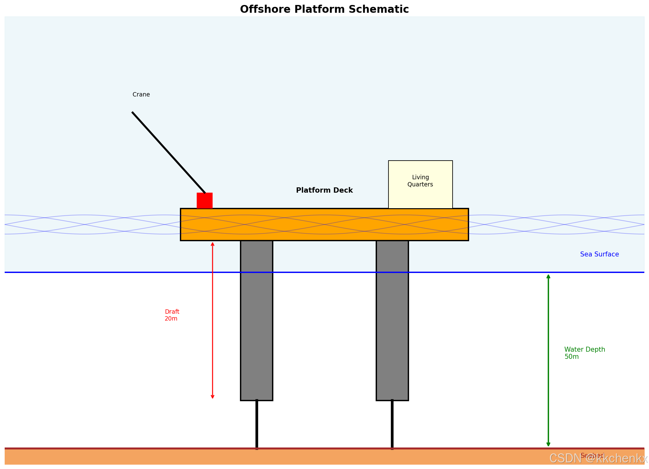
# ============ 仿真5: 海洋平台示意图 ============
print("\n正在生成海洋平台示意图...")
fig, ax = plt.subplots(figsize=(14, 12))
ax.set_xlim(-100, 100)
ax.set_ylim(-60, 80)
ax.set_aspect('equal')
ax.axis('off')
ax.set_title('Offshore Platform Schematic', fontsize=16, fontweight='bold')
# 海平面
ax.axhline(y=0, color='blue', linewidth=2, linestyle='-')
ax.fill_between([-100, 100], [0, 0], [80, 80], alpha=0.2, color='lightblue')
ax.annotate('Sea Surface', xy=(80, 5), fontsize=10, color='blue')
# 平台立柱
for i, angle in enumerate([np.pi/4, 3*np.pi/4, 5*np.pi/4, 7*np.pi/4]):
x_col = 30 * np.cos(angle)
y_bottom = -40
y_top = 10
column = Rectangle((x_col-5, y_bottom), 10, y_top-y_bottom,
fill=True, facecolor='gray', edgecolor='black', linewidth=2)
ax.add_patch(column)
# 平台甲板
deck = Rectangle((-45, 10), 90, 10, fill=True, facecolor='orange',
edgecolor='black', linewidth=2)
ax.add_patch(deck)
ax.annotate('Platform Deck', xy=(0, 25), ha='center', fontsize=11, fontweight='bold')
# 生活模块
living_quarters = Rectangle((20, 20), 20, 15, fill=True, facecolor='lightyellow',
edgecolor='black', linewidth=1)
ax.add_patch(living_quarters)
ax.annotate('Living\nQuarters', xy=(30, 27), ha='center', fontsize=9)
# 起重机
crane_base = Rectangle((-40, 20), 5, 5, fill=True, facecolor='red')
ax.add_patch(crane_base)
ax.plot([-37.5, -60], [25, 50], 'k-', linewidth=3)
ax.annotate('Crane', xy=(-60, 55), fontsize=9)
# 桩腿(水下部分)
for i, angle in enumerate([np.pi/4, 3*np.pi/4, 5*np.pi/4, 7*np.pi/4]):
x_col = 30 * np.cos(angle)
ax.plot([x_col, x_col], [-40, -55], 'k-', linewidth=4)
# 海床
ax.axhline(y=-55, color='brown', linewidth=3)
ax.fill_between([-100, 100], [-60, -60], [-55, -55], color='sandybrown')
ax.annotate('Seabed', xy=(80, -58), fontsize=10, color='brown')
# 波浪示意
x_wave = np.linspace(-100, 100, 200)
for t_wave in [0, np.pi/2, np.pi, 3*np.pi/2]:
y_wave = 3 * np.cos(2 * np.pi * x_wave / 100 + t_wave)
ax.plot(x_wave, y_wave + 15, 'b-', alpha=0.3, linewidth=1)
# 水深标注
ax.annotate('', xy=(70, 0), xytext=(70, -55),
arrowprops=dict(arrowstyle='<->', color='green', lw=2))
ax.annotate('Water Depth\n50m', xy=(75, -27), fontsize=10, color='green')
# 立柱标注
ax.annotate('', xy=(-35, -40), xytext=(-35, 10),
arrowprops=dict(arrowstyle='<->', color='red', lw=1.5))
ax.annotate('Draft\n20m', xy=(-50, -15), fontsize=9, color='red')
plt.tight_layout()
plt.savefig(f'{output_dir}/platform_schematic.png', dpi=150, bbox_inches='tight')
plt.close()
print("✓ 海洋平台示意图已保存")
print("\n" + "=" * 60)
print("所有仿真完成!")
print(f"输出目录: {output_dir}")
print("=" * 60)
# 打印水动力参数摘要
print("\n【海洋平台水动力参数摘要】")
print("-" * 40)
print(f"波浪参数:")
print(f" 波高: {wave.H} m")
print(f" 周期: {wave.T} s")
print(f" 波长: {wave.L:.1f} m")
print(f" 水深: {wave.d} m")
print("-" * 40)
print(f"平台参数:")
print(f" 质量: {platform.mass:,} kg")
print(f" 吃水: {platform.draft} m")
print(f" 立柱数: {platform.n_columns}")
print(f" 立柱直径: {platform.D_column} m")
print("-" * 40)
print(f"系泊系统:")
print(f" 系泊线数: {mooring.n_lines}")
print(f" 系泊线长度: {mooring.L} m")
print(f" 锚点半径: {mooring.anchor_radius} m")
print("-" * 40)
3. 结果分析
3.1 波浪特性
仿真结果显示了线性波浪理论的关键特征:
-
波面形状:波面呈余弦曲线,随时间向前传播。
-
水质点运动:水质点作椭圆运动,表面为圆形,随深度增加椭圆逐渐扁平。
-
色散关系:波长随周期增加而增加,深水波和浅水波有不同的传播特性。
3.2 Morison力特性
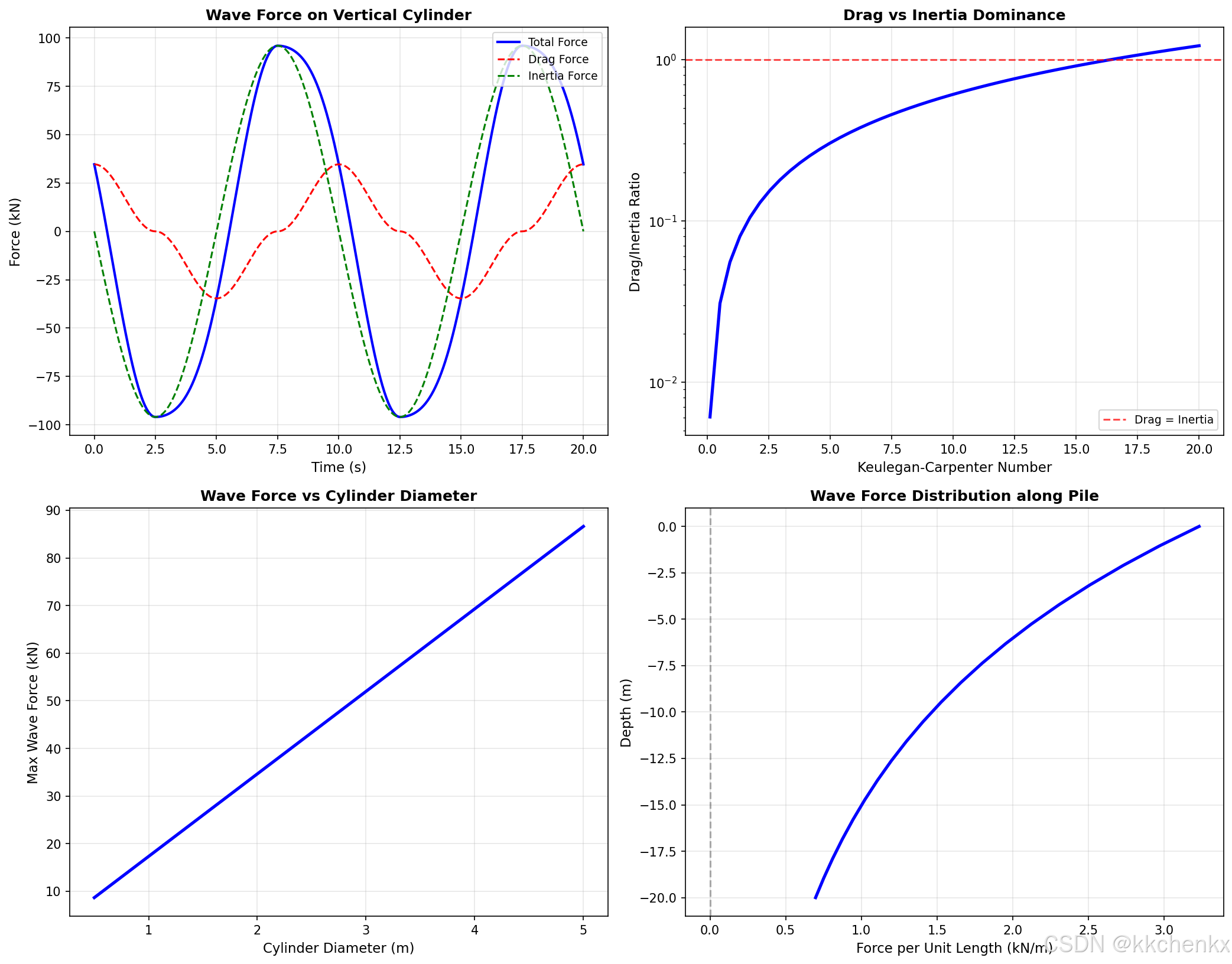
Morison方程适用于小尺度结构:
-
阻力与惯性力:在小KC数时惯性力主导,大KC数时阻力主导。
-
沿桩身分布:波浪力沿桩身分布不均匀,最大力出现在波面附近。
-
直径影响:波浪力随直径增加而增加,但增加速率逐渐减缓。
3.3 平台运动响应
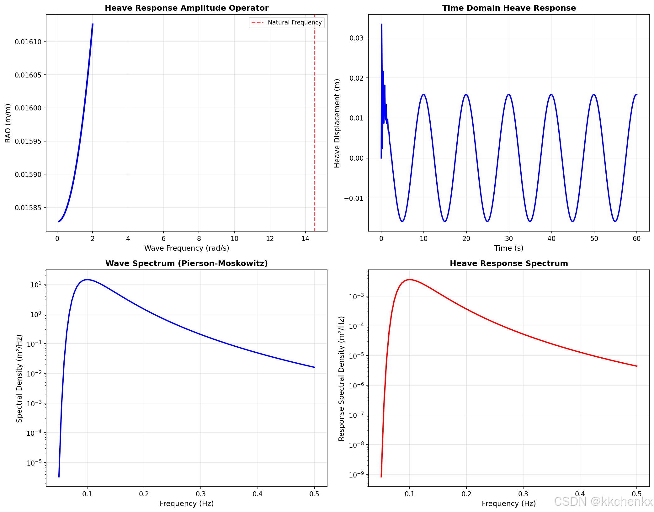
平台运动响应反映了其水动力特性:
-
RAO曲线:响应幅值算子在固有频率处出现峰值,需要避免与波浪频率重合。
-
时域响应:平台运动呈现周期性,与波浪激励频率一致。
-
响应谱:通过波浪谱和RAO可以计算平台运动的统计特性。
3.4 系泊系统
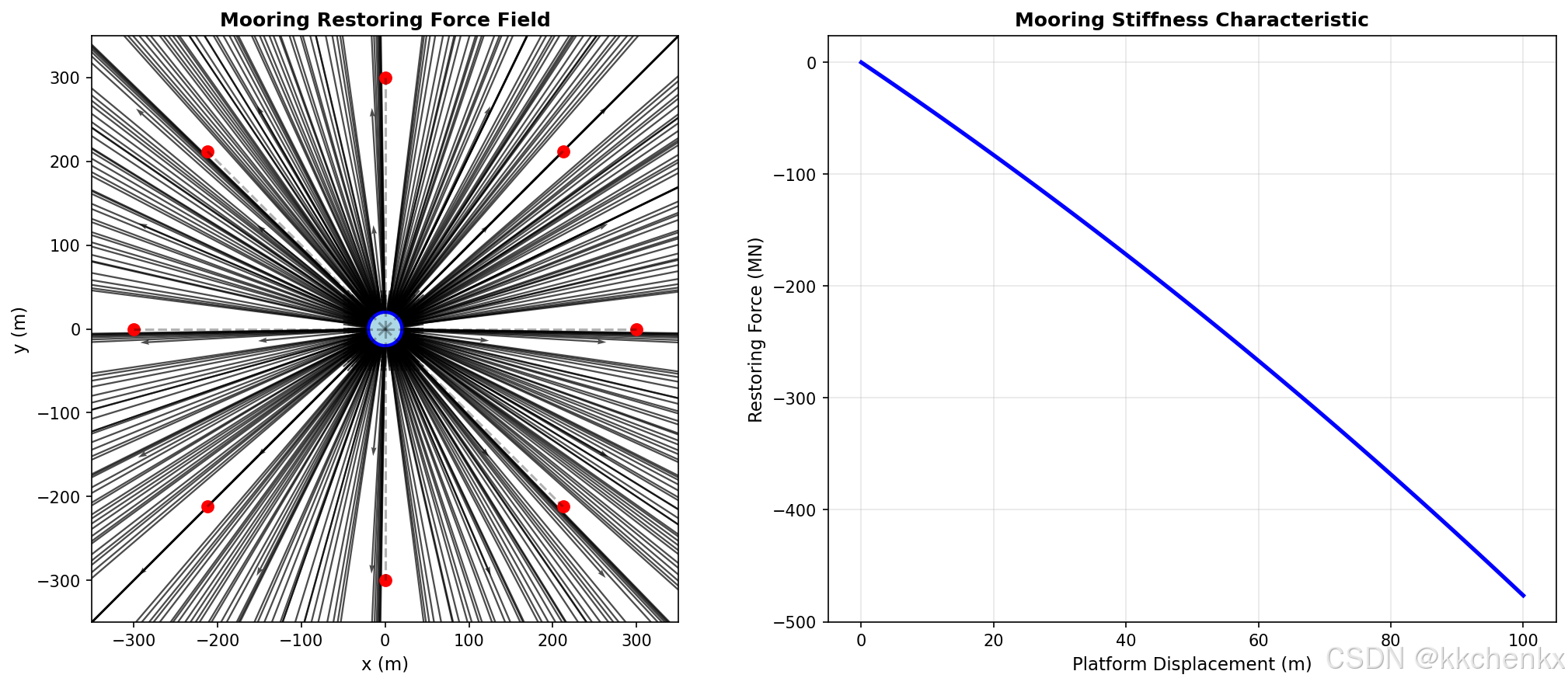
系泊系统提供水平面内的恢复力:
-
恢复力特性:系泊恢复力随位移增加而增加,呈非线性特性。
-
对称性:多根系泊线对称布置,提供各向同性的恢复力。
-
设计考虑:需要保证系泊系统在极端海况下不发生失效。
4. 扩展与应用
4.1 不同平台类型
不同类型的海洋平台有各自的特点:
-
固定式平台:适用于浅水,通过桩基固定于海床。
-
半潜式平台:通过浮筒和立柱提供浮力,运动响应较小。
-
FPSO:浮式生产储油船,需要单点系泊系统。
-
** Spar平台**:重心低于浮心,具有天然的稳定性。
4.2 环境载荷
除了波浪,还需要考虑其他环境载荷:
-
风载荷:对平台上部结构产生作用力。
-
流载荷:海流对结构产生拖曳力。
-
冰载荷:在寒冷海域需要考虑海冰的作用。
-
地震载荷:在地震活跃区域需要考虑地震作用。
4.3 工程应用建议
-
设计阶段:
- 进行详细的水动力分析
- 优化平台几何形状
- 设计合适的系泊系统
-
安装阶段:
- 制定详细的安装方案
- 考虑安装期间的海况限制
- 进行拖航分析
-
运营阶段:
- 监测平台运动和应力
- 定期检查系泊系统
- 评估疲劳寿命
5. 总结
本教程通过Python仿真详细展示了海洋平台的水动力学特性,包括:
- 波浪理论:建立了线性波浪模型,分析了波浪传播特性
- 波浪力计算:使用Morison方程计算了小尺度结构的波浪力
- 运动响应:分析了平台的垂荡响应和RAO特性
- 系泊系统:建立了系泊恢复力模型,分析了系泊特性
这些仿真方法为海洋平台的设计、安全评估和运营优化提供了理论基础和分析工具。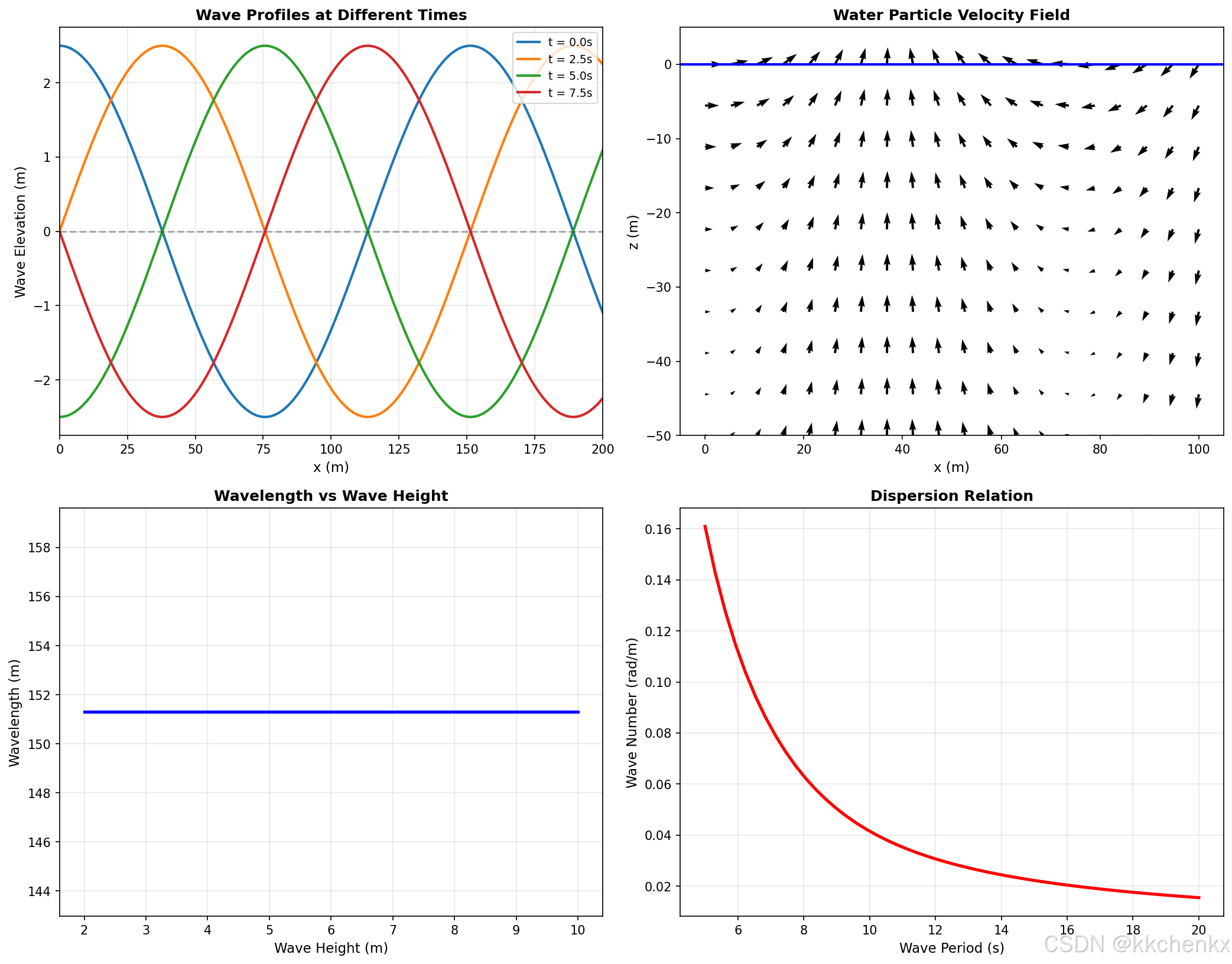

有“AI”的1024 = 2048,欢迎大家加入2048 AI社区
更多推荐

 6
6 0
0- 0


 已为社区贡献8条内容

所有评论(0)