第8篇:Attention Is All You Need——从Seq2Seq到Transformer的飞跃
《Attention Is All You Need》论文提出Transformer架构,彻底改变了序列建模方式。该模型摒弃传统RNN结构,完全基于注意力机制,实现了并行计算和长距离依赖捕捉。核心创新包括:自注意力机制使每个位置直接关注全局信息;多头注意力从多个角度提取特征;位置编码解决序列顺序问题。Transformer架构分为编码器和解码器,通过残差连接和层归一化优化训练。这一突破性设计为BE
第8篇:Attention Is All You Need——从Seq2Seq到Transformer的飞跃
一、一个颠覆性的标题
2017年6月,Google的研究团队发表了一篇论文,标题简单、直接、“暴力”:
“Attention Is All You Need”
这句话的潜台词是:我们不需要RNN,不需要CNN,只需要Attention机制,就能构建强大的序列模型。
当时的主流观点:
- RNN/LSTM是序列建模的标准
- 注意力只是辅助工具(帮RNN"看"到重要部分)
- 并行计算是不可能的(序列必须一步一步处理)
这篇论文彻底颠覆了这些认知,开启了大模型时代。
二、RNN的瓶颈:为什么必须抛弃循环?
2.1 无法并行计算
RNN的处理是顺序的:
时刻1 → 时刻2 → 时刻3 → ... → 时刻100
要计算时刻100的隐藏状态,必须等前面99步全部完成。这意味着:
- 100个时间步 = 100个串行操作
- GPU的并行计算能力完全浪费
- 训练长序列极其缓慢
2.2 长距离依赖的局限
即使LSTM有门控机制,信息从时刻1传到时刻100,仍然需要经过99次矩阵运算。梯度消失问题缓解但未根除。
2.3 计算复杂度对比
| 操作 | RNN | Transformer |
|---|---|---|
| 单步计算 | O ( d 2 ) O(d^2) O(d2) | O ( d 2 ) O(d^2) O(d2) |
| 序列长度 n n n | O ( n ⋅ d 2 ) O(n \cdot d^2) O(n⋅d2) | O ( n 2 ⋅ d ) O(n^2 \cdot d) O(n2⋅d) |
| 并行度 | 1(串行) | n n n(完全并行) |
关键洞察:Transformer用 O ( n 2 ) O(n^2) O(n2)的复杂度换取了完全并行,在GPU上实际训练速度提升10-100倍。
三、Attention机制:从"看"到"关注"
3.1 直觉:人类的注意力
读这句话时:
“猫坐在垫子上,因为它很温暖。”
你的注意力流程:
- 读到"它"时,回看前面的"垫子"或"猫"
- 根据"温暖"的线索,确定"它"指"垫子"
- 不需要逐字重读,直接跳转到相关信息
Attention机制就是让这个"回看"和"跳转"变得可计算。
3.2 Query, Key, Value:注意力三要素
想象一个数据库查询系统:
| 概念 | 类比 | 作用 |
|---|---|---|
| Query | 你的搜索关键词 | 表示"我要找什么" |
| Key | 数据库索引 | 表示"每个条目的标签" |
| Value | 数据库内容 | 表示"每个条目的实际信息" |
计算过程:
- Query与所有Key计算相似度(点积)
- 相似度归一化为权重(Softmax)
- 用权重对Value加权求和,得到输出
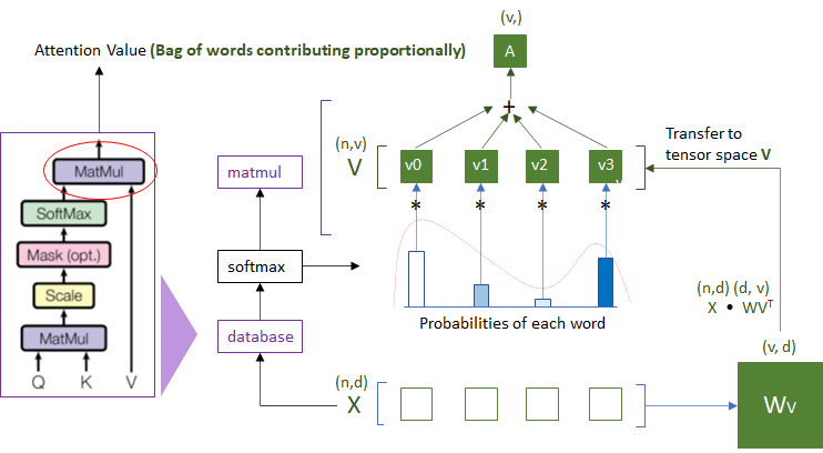
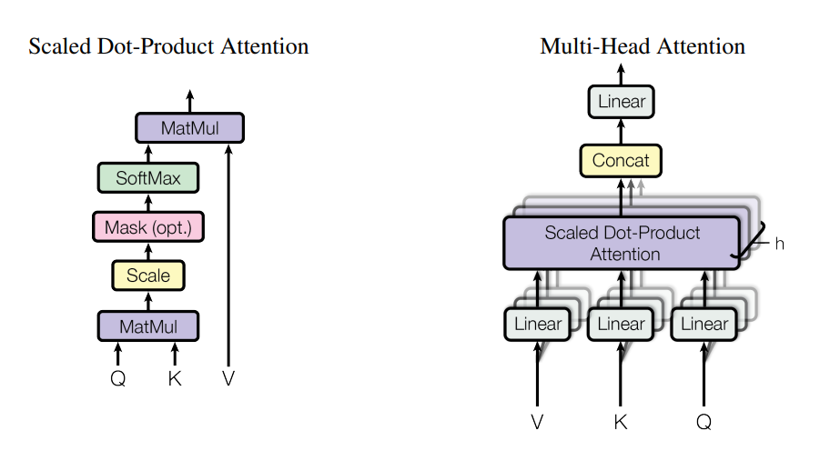
3.3 Scaled Dot-Product Attention
数学公式:
Attention ( Q , K , V ) = softmax ( Q K T d k ) V \text{Attention}(Q, K, V) = \text{softmax}\left(\frac{QK^T}{\sqrt{d_k}}\right)V Attention(Q,K,V)=softmax(dkQKT)V
一步步推导:
Step 1:计算相似度矩阵
S = Q K T S = QK^T S=QKT
S i j S_{ij} Sij表示第 i i i个Query与第 j j j个Key的相似度。
Step 2:缩放(Scaling)
S ~ = S d k \tilde{S} = \frac{S}{\sqrt{d_k}} S~=dkS
为什么除以 d k \sqrt{d_k} dk?
- 当 d k d_k dk很大时,点积的方差会很大
- Softmax在输入很大时梯度极小(饱和)
- 缩放保持数值稳定,梯度健康
Step 3:归一化(Softmax)
A = softmax ( S ~ ) A = \text{softmax}(\tilde{S}) A=softmax(S~)
A i j A_{ij} Aij表示第 i i i个位置对第 j j j个位置的注意力权重,和为1。
Step 4:加权求和
Output = A V \text{Output} = AV Output=AV
每个输出位置是所有Value的加权平均,权重由注意力决定。
四、Self-Attention:自己关注自己
4.1 核心思想
传统的Attention是跨序列的(如机器翻译中,Decoder关注Encoder)。
Self-Attention是序列内部的:每个位置关注序列中的所有位置(包括自己)。
为什么有效?
- 捕捉长距离依赖:位置1可以直接"看"到位置100
- 并行计算:所有位置的注意力同时计算
- 可解释性强:注意力权重显示模型"关注"哪里
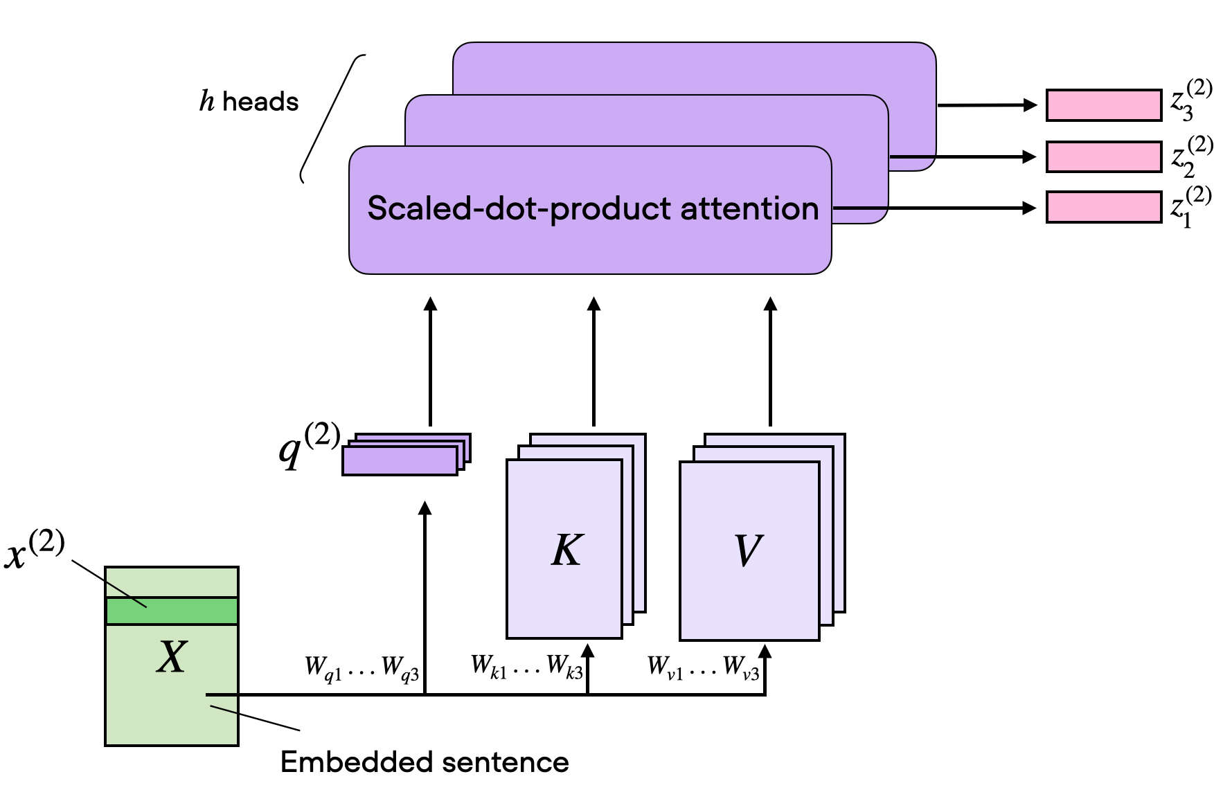
4.2 从输入到Q, K, V
输入向量 X X X通过三个不同的线性变换得到Q, K, V:
Q = X W Q , K = X W K , V = X W V Q = XW_Q, \quad K = XW_K, \quad V = XW_V Q=XWQ,K=XWK,V=XWV
其中 W Q , W K , W V W_Q, W_K, W_V WQ,WK,WV是可学习的参数矩阵。
维度说明:
- 输入 X X X: ( n , d model ) (n, d_{\text{model}}) (n,dmodel), n n n是序列长度
- W Q , W K W_Q, W_K WQ,WK: ( d model , d k ) (d_{\text{model}}, d_k) (dmodel,dk)
- W V W_V WV: ( d model , d v ) (d_{\text{model}}, d_v) (dmodel,dv)
- 输出: ( n , d v ) (n, d_v) (n,dv)
通常 d k = d v = d model / h d_k = d_v = d_{\text{model}} / h dk=dv=dmodel/h,其中 h h h是注意力头数。
五、Multi-Head Attention:多头并行的智慧
5.1 为什么需要多头?
单一的Attention可能只捕捉一种关系:
- "它"指代什么?
- 语法结构?
- 语义相似?
多头机制:让模型同时从多个"角度"关注信息。
5.2 计算过程
输入X
    │
    ├──→ Head 1: Q1, K1, V1 → Attention1
    ├──→ Head 2: Q2, K2, V2 → Attention2
    ...
    └──→ Head h: Qh, Kh, Vh → Attentionh

    ↓
拼接所有头的输出 → 线性变换 → 最终输出
数学表达:
MultiHead ( Q , K , V ) = Concat ( head 1 , . . . , head h ) W O \text{MultiHead}(Q, K, V) = \text{Concat}(\text{head}_1, ..., \text{head}_h)W^O MultiHead(Q,K,V)=Concat(head1,...,headh)WO
其中:
head i = Attention ( X W Q i , X W K i , X W V i ) \text{head}_i = \text{Attention}(XW_{Q_i}, XW_{K_i}, XW_{V_i}) headi=Attention(XWQi,XWKi,XWVi)
5.3 可视化理解
| 头 | 学到的模式 | 示例 |
|---|---|---|
| Head 1 | 指代消解 | “它” → “猫” |
| Head 2 | 句法关系 | 主语-谓语-宾语 |
| Head 3 | 语义相似 | “国王”-“女王”(性别) |
| Head 4 | 位置邻近 | 相邻词的关系 |
六、位置编码:给序列加上"顺序"
6.1 为什么需要位置编码?
Attention是位置无关的:
- "猫追狗"和"狗追猫"的Q, K, V计算完全一样
- 模型不知道哪个词在前,哪个在后
必须显式注入位置信息。
6.2 正弦位置编码
Transformer使用的位置编码:
P E ( p o s , 2 i ) = sin ( p o s 10000 2 i / d model ) PE_{(pos, 2i)} = \sin\left(\frac{pos}{10000^{2i/d_{\text{model}}}}\right) PE(pos,2i)=sin(100002i/dmodelpos)
P E ( p o s , 2 i + 1 ) = cos ( p o s 10000 2 i / d model ) PE_{(pos, 2i+1)} = \cos\left(\frac{pos}{10000^{2i/d_{\text{model}}}}\right) PE(pos,2i+1)=cos(100002i/dmodelpos)
直观理解:
| 维度 | 波长 | 编码特征 |
|---|---|---|
| 低维度( 2 i 2i 2i小) | 短 | 精确位置信息 |
| 高维度( 2 i 2i 2i大) | 长 | 相对位置关系 |
为什么用正弦/余弦?
- 唯一性:每个位置有唯一编码
- 相对位置: P E p o s + k PE_{pos+k} PEpos+k可以用 P E p o s PE_{pos} PEpos线性表示
- 外推性:可以处理训练时未见过的长度
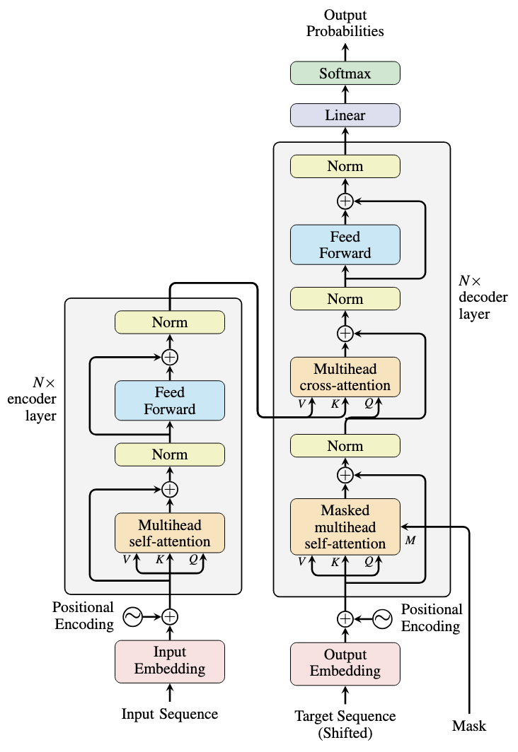
七、Transformer完整架构
7.1 Encoder(编码器)
输入嵌入 + 位置编码
    ↓
Multi-Head Self-Attention
    ↓
Add & Norm(残差连接 + LayerNorm)
    ↓
Feed Forward(全连接前馈网络)
    ↓
Add & Norm
    ↓
重复N次(通常N=6或12)
关键组件:
- 残差连接(Residual Connection): x + Sublayer ( x ) x + \text{Sublayer}(x) x+Sublayer(x),缓解梯度消失
- Layer Normalization:对每个样本的特征归一化,稳定训练
- Feed Forward:两个线性变换夹一个ReLU, F F N ( x ) = max ( 0 , x W 1 + b 1 ) W 2 + b 2 FFN(x) = \max(0, xW_1 + b_1)W_2 + b_2 FFN(x)=max(0,xW1+b1)W2+b2
7.2 Decoder(解码器)
输入嵌入 + 位置编码
    ↓
Masked Multi-Head Self-Attention(掩码,防止看到未来)
    ↓
Add & Norm
    ↓
Multi-Head Cross-Attention(关注Encoder输出)
    ↓
Add & Norm
    ↓
Feed Forward
    ↓
Add & Norm
    ↓
重复N次
    ↓
Linear + Softmax → 输出概率
Masked Attention:位置 i i i只能关注位置 ≤ i \leq i ≤i,保证自回归生成。
7.3 BERT vs GPT:两种Transformer变体
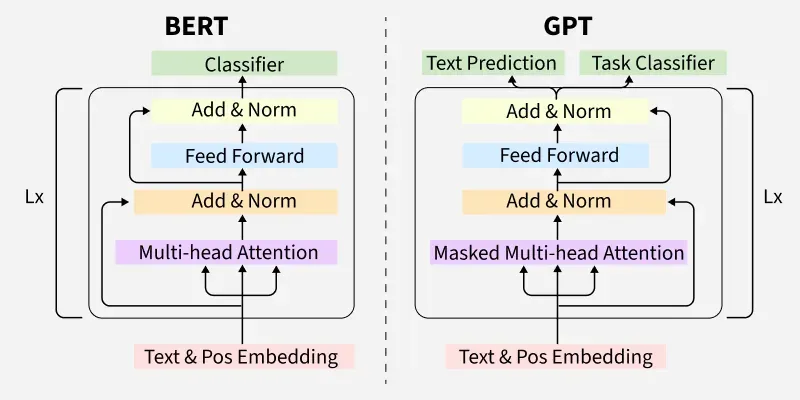
| 特性 | BERT | GPT |
|---|---|---|
| 架构 | Encoder-only | Decoder-only |
| 训练目标 | 掩码语言模型(MLM) | 自回归语言建模 |
| 方向 | 双向(看上下文) | 单向(看前文) |
| 典型应用 | 文本理解、分类 | 文本生成 |
| 代表模型 | BERT, RoBERTa | GPT-2/3/4, ChatGPT |
八、Python实现:简化版Transformer
import numpy as np
import tensorflow as tf
from tensorflow import keras
from tensorflow.keras import layers

# 位置编码
class PositionalEncoding(layers.Layer):
    def __init__(self, max_seq_len, d_model):
        super().__init__()
        self.d_model = d_model

        # 创建位置编码矩阵
        pe = np.zeros((max_seq_len, d_model))
        position = np.arange(0, max_seq_len)[:, np.newaxis]
        div_term = np.exp(np.arange(0, d_model, 2) *
                         -(np.log(10000.0) / d_model))

        pe[:, 0::2] = np.sin(position * div_term)
        pe[:, 1::2] = np.cos(position * div_term)

        self.pe = tf.constant(pe[np.newaxis, ...], dtype=tf.float32)

    def call(self, x):
        seq_len = tf.shape(x)[1]
        return x + self.pe[:, :seq_len, :]

# 多头注意力
class MultiHeadAttention(layers.Layer):
    def __init__(self, d_model, num_heads):
        super().__init__()
        self.num_heads = num_heads
        self.d_model = d_model
        self.depth = d_model // num_heads

        self.wq = layers.Dense(d_model)
        self.wk = layers.Dense(d_model)
        self.wv = layers.Dense(d_model)
        self.dense = layers.Dense(d_model)

    def split_heads(self, x, batch_size):
        x = tf.reshape(x, (batch_size, -1, self.num_heads, self.depth))
        return tf.transpose(x, perm=[0, 2, 1, 3])

    def call(self, v, k, q, mask=None):
        batch_size = tf.shape(q)[0]

        q = self.wq(q)
        k = self.wk(k)
        v = self.wv(v)

        q = self.split_heads(q, batch_size)
        k = self.split_heads(k, batch_size)
        v = self.split_heads(v, batch_size)

        # Scaled dot-product attention
        matmul_qk = tf.matmul(q, k, transpose_b=True)
        dk = tf.cast(tf.shape(k)[-1], tf.float32)
        scaled_attention_logits = matmul_qk / tf.math.sqrt(dk)

        if mask is not None:
            scaled_attention_logits += (mask * -1e9)

        attention_weights = tf.nn.softmax(scaled_attention_logits, axis=-1)
        output = tf.matmul(attention_weights, v)

        output = tf.transpose(output, perm=[0, 2, 1, 3])
        concat_attention = tf.reshape(output, (batch_size, -1, self.d_model))

        output = self.dense(concat_attention)
        return output, attention_weights

# 前馈网络
class FeedForward(layers.Layer):
    def __init__(self, d_model, d_ff):
        super().__init__()
        self.dense1 = layers.Dense(d_ff, activation='relu')
        self.dense2 = layers.Dense(d_model)

    def call(self, x):
        return self.dense2(self.dense1(x))

# Transformer Encoder层
class EncoderLayer(layers.Layer):
    def __init__(self, d_model, num_heads, d_ff, dropout_rate=0.1):
        super().__init__()
        self.mha = MultiHeadAttention(d_model, num_heads)
        self.ffn = FeedForward(d_model, d_ff)

        self.layernorm1 = layers.LayerNormalization(epsilon=1e-6)
        self.layernorm2 = layers.LayerNormalization(epsilon=1e-6)

        self.dropout1 = layers.Dropout(dropout_rate)
        self.dropout2 = layers.Dropout(dropout_rate)

    def call(self, x, training, mask=None):
        # Multi-Head Self-Attention
        attn_output, _ = self.mha(x, x, x, mask)
        attn_output = self.dropout1(attn_output, training=training)
        out1 = self.layernorm1(x + attn_output)  # 残差连接

        # Feed Forward
        ffn_output = self.ffn(out1)
        ffn_output = self.dropout2(ffn_output, training=training)
        out2 = self.layernorm2(out1 + ffn_output)  # 残差连接

        return out2

# 完整的Transformer Encoder
class TransformerEncoder(keras.Model):
    def __init__(self, num_layers, d_model, num_heads, d_ff,
                 input_vocab_size, max_seq_len, dropout_rate=0.1):
        super().__init__()

        self.d_model = d_model
        self.num_layers = num_layers

        self.embedding = layers.Embedding(input_vocab_size, d_model)
        self.pos_encoding = PositionalEncoding(max_seq_len, d_model)
        self.dropout = layers.Dropout(dropout_rate)

        self.enc_layers = [EncoderLayer(d_model, num_heads, d_ff, dropout_rate)
                          for _ in range(num_layers)]

    def call(self, x, training, mask=None):
        seq_len = tf.shape(x)[1]

        # 嵌入 + 位置编码
        x = self.embedding(x)
        x *= tf.math.sqrt(tf.cast(self.d_model, tf.float32))
        x = self.pos_encoding(x)
        x = self.dropout(x, training=training)

        # 通过所有Encoder层
        for i in range(self.num_layers):
            x = self.enc_layers[i](x, training, mask)

        return x

# 测试
print("构建Transformer Encoder...")
encoder = TransformerEncoder(
    num_layers=2,
    d_model=128,
    num_heads=8,
    d_ff=512,
    input_vocab_size=10000,
    max_seq_len=100
)

# 测试输入
test_input = tf.random.uniform((32, 50), dtype=tf.int32, maxval=10000)
output = encoder(test_input, training=False)

print(f"输入形状: {test_input.shape}")
print(f"输出形状: {output.shape}")
print("\nTransformer Encoder构建成功!")
九、C/C++实现:注意力计算核心
#include <stdio.h>
#include <stdlib.h>
#include <math.h>
#include <string.h>

#define SEQ_LEN 4
#define D_MODEL 8
#define D_K 4  // D_MODEL / NUM_HEADS

// Softmax函数
void softmax(double* x, int n) {
    double max_val = x[0];
    for (int i = 1; i < n; i++) {
        if (x[i] > max_val) max_val = x[i];
    }

    double sum = 0.0;
    for (int i = 0; i < n; i++) {
        x[i] = exp(x[i] - max_val);
        sum += x[i];
    }

    for (int i = 0; i < n; i++) {
        x[i] /= sum;
    }
}

// 矩阵乘法:C = A * B^T
void matmul_transpose_b(double A[SEQ_LEN][D_K], double B[SEQ_LEN][D_K],
                        double C[SEQ_LEN][SEQ_LEN]) {
    for (int i = 0; i < SEQ_LEN; i++) {
        for (int j = 0; j < SEQ_LEN; j++) {
            C[i][j] = 0.0;
            for (int k = 0; k < D_K; k++) {
                C[i][j] += A[i][k] * B[j][k];
            }
        }
    }
}

// 矩阵乘法:C = A * B
void matmul(double A[SEQ_LEN][SEQ_LEN], double B[SEQ_LEN][D_K],
            double C[SEQ_LEN][D_K]) {
    for (int i = 0; i < SEQ_LEN; i++) {
        for (int j = 0; j < D_K; j++) {
            C[i][j] = 0.0;
            for (int k = 0; k < SEQ_LEN; k++) {
                C[i][j] += A[i][k] * B[k][j];
            }
        }
    }
}

// Scaled Dot-Product Attention
void scaled_dot_product_attention(
    double Q[SEQ_LEN][D_K],
    double K[SEQ_LEN][D_K],
    double V[SEQ_LEN][D_K],
    double output[SEQ_LEN][D_K],
    double attention_weights[SEQ_LEN][SEQ_LEN]
) {
    double scores[SEQ_LEN][SEQ_LEN];

    // 计算 Q * K^T
    matmul_transpose_b(Q, K, scores);

    // 缩放
    double scale = sqrt(D_K);
    for (int i = 0; i < SEQ_LEN; i++) {
        for (int j = 0; j < SEQ_LEN; j++) {
            scores[i][j] /= scale;
        }
    }

    // Softmax(按行)
    for (int i = 0; i < SEQ_LEN; i++) {
        softmax(scores[i], SEQ_LEN);
        memcpy(attention_weights[i], scores[i], sizeof(scores[i]));
    }

    // 乘以 V
    matmul(scores, V, output);
}

int main() {
    printf("Scaled Dot-Product Attention演示\n");
    printf("================================\n");
    printf("序列长度: %d\n", SEQ_LEN);
    printf("模型维度: %d\n", D_MODEL);
    printf("Key/Query维度: %d\n\n", D_K);

    // 简化的Q, K, V(实际应从输入线性变换得到)
    double Q[SEQ_LEN][D_K] = {
        {1.0, 0.0, 0.0, 0.0},  // "我"
        {0.0, 1.0, 0.0, 0.0},  // "爱"
        {0.0, 0.0, 1.0, 0.0},  // "深度"
        {0.0, 0.0, 0.0, 1.0}   // "学习"
    };

    double K[SEQ_LEN][D_K] = {
        {1.0, 0.0, 0.0, 0.0},
        {0.0, 1.0, 0.0, 0.0},
        {0.0, 0.0, 1.0, 0.0},
        {0.0, 0.0, 0.0, 1.0}
    };

    double V[SEQ_LEN][D_K] = {
        {1.0, 0.0, 0.0, 0.0},
        {0.0, 1.0, 0.0, 0.0},
        {0.0, 0.0, 1.0, 0.0},
        {0.0, 0.0, 0.0, 1.0}
    };

    double output[SEQ_LEN][D_K];
    double attention[SEQ_LEN][SEQ_LEN];

    scaled_dot_product_attention(Q, K, V, output, attention);

    printf("注意力权重矩阵:\n");
    printf("        我    爱   深度  学习\n");
    for (int i = 0; i < SEQ_LEN; i++) {
        printf("位置%d: ", i);
        for (int j = 0; j < SEQ_LEN; j++) {
            printf("%.3f ", attention[i][j]);
        }
        printf("\n");
    }

    printf("\n关键观察:\n");
    printf("1. 对角线值较高:每个位置最关注自己\n");
    printf("2. 非对角线值:关注其他位置的程度\n");
    printf("3. 每行和为1:Softmax归一化结果\n");
    printf("\n在实际Transformer中,Q/K/V通过线性变换从输入得到,\n");
    printf("注意力权重会学习到词语间的语义关系。\n");

    return 0;
}
编译运行:
gcc attention.c -o attention -lm
./attention
十、Java实现:Multi-Head Attention
import java.util.*;

public class TransformerAttention {

    // 矩阵工具类
    static class Matrix {
        static double[][] multiply(double[][] a, double[][] b) {
            int m = a.length, n = b[0].length, p = b.length;
            double[][] c = new double[m][n];
            for (int i = 0; i < m; i++) {
                for (int j = 0; j < n; j++) {
                    for (int k = 0; k < p; k++) {
                        c[i][j] += a[i][k] * b[k][j];
                    }
                }
            }
            return c;
        }

        static double[][] transpose(double[][] a) {
            int m = a.length, n = a[0].length;
            double[][] t = new double[n][m];
            for (int i = 0; i < m; i++) {
                for (int j = 0; j < n; j++) {
                    t[j][i] = a[i][j];
                }
            }
            return t;
        }

        static void softmax(double[][] x) {
            for (int i = 0; i < x.length; i++) {
                double max = x[i][0];
                for (int j = 1; j < x[i].length; j++) {
                    if (x[i][j] > max) max = x[i][j];
                }

                double sum = 0.0;
                for (int j = 0; j < x[i].length; j++) {
                    x[i][j] = Math.exp(x[i][j] - max);
                    sum += x[i][j];
                }

                for (int j = 0; j < x[i].length; j++) {
                    x[i][j] /= sum;
                }
            }
        }

        static void print(double[][] m, String name) {
            System.out.println("\n" + name + ":");
            for (double[] row : m) {
                for (double val : row) {
                    System.out.printf("%.3f ", val);
                }
                System.out.println();
            }
        }
    }

    // Multi-Head Attention
    static class MultiHeadAttention {
        int numHeads, dModel, dK;
        Random rand;

        // 权重矩阵(简化:每个头共享,实际应独立)
        double[][] Wq, Wk, Wv, Wo;

        public MultiHeadAttention(int numHeads, int dModel) {
            this.numHeads = numHeads;
            this.dModel = dModel;
            this.dK = dModel / numHeads;
            this.rand = new Random(42);

            // Xavier初始化
            double scale = Math.sqrt(2.0 / dModel);

            Wq = new double[dModel][dModel];
            Wk = new double[dModel][dModel];
            Wv = new double[dModel][dModel];
            Wo = new double[dModel][dModel];

            for (int i = 0; i < dModel; i++) {
                for (int j = 0; j < dModel; j++) {
                    Wq[i][j] = (rand.nextDouble() - 0.5) * 2 * scale;
                    Wk[i][j] = (rand.nextDouble() - 0.5) * 2 * scale;
                    Wv[i][j] = (rand.nextDouble() - 0.5) * 2 * scale;
                    Wo[i][j] = (rand.nextDouble() - 0.5) * 2 * scale;
                }
            }
        }

        public double[][] forward(double[][] x) {
            int seqLen = x.length;

            // 线性变换得到Q, K, V
            double[][] Q = Matrix.multiply(x, Wq);
            double[][] K = Matrix.multiply(x, Wk);
            double[][] V = Matrix.multiply(x, Wv);

            // Scaled dot-product attention
            double[][] Kt = Matrix.transpose(K);
            double[][] scores = Matrix.multiply(Q, Kt);

            // 缩放
            double scale = Math.sqrt(dK);
            for (int i = 0; i < seqLen; i++) {
                for (int j = 0; j < seqLen; j++) {
                    scores[i][j] /= scale;
                }
            }

            // Softmax
            Matrix.softmax(scores);

            // 注意力输出
            double[][] attnOutput = Matrix.multiply(scores, V);

            // 输出线性变换
            return Matrix.multiply(attnOutput, Wo);
        }
    }

    public static void main(String[] args) {
        System.out.println("Multi-Head Attention演示");
        System.out.println("========================\n");

        int seqLen = 4;
        int dModel = 8;
        int numHeads = 2;

        System.out.println("序列长度: " + seqLen);
        System.out.println("模型维度: " + dModel);
        System.out.println("注意力头数: " + numHeads);
        System.out.println("每头维度: " + (dModel / numHeads) + "\n");

        // 模拟输入(4个token,每个8维)
        double[][] x = {
            {1, 0, 0, 0, 0, 0, 0, 0},  // token 1
            {0, 1, 0, 0, 0, 0, 0, 0},  // token 2
            {0, 0, 1, 0, 0, 0, 0, 0},  // token 3
            {0, 0, 0, 1, 0, 0, 0, 0}   // token 4
        };

        MultiHeadAttention mha = new MultiHeadAttention(numHeads, dModel);
        double[][] output = mha.forward(x);

        Matrix.print(x, "输入");
        Matrix.print(output, "Multi-Head Attention输出");

        System.out.println("\n关键观察:");
        System.out.println("1. 输出形状与输入相同: (" + output.length + ", " + output[0].length + ")");
        System.out.println("2. 每个位置的输出融合了全序列的信息");
        System.out.println("3. 多头机制让模型从多个角度捕捉关系");
        System.out.println("\n在完整Transformer中,此输出会经过:");
        System.out.println("  残差连接 → LayerNorm → Feed Forward → 下一层");
    }
}
十一、Transformer的影响:大模型时代
11.1 从Transformer到GPT/BERT
| 时间 | 模型 | 参数量 | 突破 |
|---|---|---|---|
| 2017 | Transformer | 65M | 提出架构 |
| 2018 | BERT/GPT-1 | 110M/117M | 预训练+微调 |
| 2019 | GPT-2 | 1.5B | 零样本能力 |
| 2020 | GPT-3 | 175B | 涌现能力 |
| 2022 | ChatGPT | 175B+ | 指令微调+RLHF |
| 2023 | GPT-4 | 未公开 | 多模态 |
11.2 为什么Transformer适合做大模型?
| 特性 | RNN | Transformer |
|---|---|---|
| 并行度 | 低(串行) | 高(完全并行) |
| 长距离依赖 | 困难 | 直接连接 |
| 可扩展性 | 差 | 好(堆叠层数) |
| 训练稳定性 | 梯度问题 | 残差连接+LayerNorm |
关键:Transformer的架构天然适合GPU并行,可以堆叠成百上千层,训练千亿参数。
十二、总结与展望
12.1 五大神经网络架构回顾
第6篇:CNN  →  空间建模,图像识别
第7篇:RNN  →  时间建模,序列处理
第8篇:Transformer →  注意力机制,并行计算
      ↓
     统一
      ↓
第9篇:GAN  →  生成模型(即将开启)
12.2 关键公式速查
| 组件 | 公式 | 作用 |
|---|---|---|
| Scaled Attention | softmax ( Q K T d k ) V \text{softmax}(\frac{QK^T}{\sqrt{d_k}})V softmax(dkQKT)V | 计算注意力权重 |
| Multi-Head | Concat ( head 1 , . . . , head h ) W O \text{Concat}(\text{head}_1, ..., \text{head}_h)W^O Concat(head1,...,headh)WO | 多头并行 |
| 位置编码 | sin ( p o s / 10000 2 i / d ) \sin(pos/10000^{2i/d}) sin(pos/100002i/d) | 注入位置信息 |
| FFN | max ( 0 , x W 1 + b 1 ) W 2 + b 2 \max(0, xW_1+b_1)W_2+b_2 max(0,xW1+b1)W2+b2 | 非线性变换 |
12.3 从理论到实践
你已经掌握了:
- 线性回归、逻辑回归(基础)
- MLP、CNN、RNN、LSTM、Transformer(五大架构)
下一步:
- GAN:生成对抗网络,创造新数据
- 实践项目:用PyTorch/TensorFlow实现完整模型
- 前沿探索:Vision Transformer、Mamba等新架构
下一篇预告:《第9篇:创造的艺术——生成对抗网络GAN与图像生成》
我们将进入深度学习的另一个分支:生成模型。GAN让两个神经网络互相博弈,创造出以假乱真的图像,开启了AI艺术创作的新纪元。
配图清单:
- 图1:Transformer完整架构图
- 图2:Query-Key-Value注意力机制
- 图3:Multi-Head Attention结构
- 图4:位置编码正弦曲线
- 图5:BERT vs GPT架构对比
全文约6500字,是深度学习五大架构的第三篇(Transformer)。从"Attention Is All You Need"到GPT-4,我们见证了深度学习最具革命性的突破。第9篇GAN,将开启生成模型的新篇章!
本文部分内容由AI编辑,可能会出现幻觉,请谨慎阅读。

有“AI”的1024 = 2048,欢迎大家加入2048 AI社区
更多推荐

 4
4 0
0- 0


 已为社区贡献3条内容

所有评论(0)