【机器学习案例-39】Kaggle案例之AI依赖与学生学业表现:数据分析与预测建模全流程
在ChatGPT、Gemini、Copilot等人工智能工具迅速普及的当下,教育领域正经历着一场前所未有的变革。人工智能辅助学习工具已经从"锦上添花"变为"日常必备",深刻影响着学生的学习方式和学术表现。然而,一个关键问题日益凸显:AI工具的使用究竟是促进学生学业成功的神奇帮手,还是削弱独立思考能力的"双刃剑"?。本文基于8000名学生的学业表现与AI使用数据,深入分析了AI依赖度对学生学习成绩的
🧑 博主简介:曾任某智慧城市类企业
算法总监,目前在美国市场的物流公司从事高级算法工程师一职,深耕人工智能领域,精通python数据挖掘、可视化、机器学习等,发表过AI相关的专利并多次在AI类比赛中获奖。CSDN人工智能领域的优质创作者,提供AI相关的技术咨询、项目开发和个性化解决方案等服务,如有需要请站内私信或者联系任意文章底部的的VX名片(ID:xf982831907)
💬 博主粉丝群介绍:① 群内初中生、高中生、本科生、研究生、博士生遍布,可互相学习,交流困惑。② 热榜top10的常客也在群里,也有数不清的万粉大佬,可以交流写作技巧,上榜经验,涨粉秘籍。③ 群内也有职场精英,大厂大佬,可交流技术、面试、找工作的经验。④ 进群免费赠送写作秘籍一份,助你由写作小白晋升为创作大佬。⑤ 进群赠送CSDN评论防封脚本,送真活跃粉丝,助你提升文章热度。有兴趣的加文末联系方式,备注自己的CSDN昵称,拉你进群,互相学习共同进步。

【机器学习案例-39】Kaggle案例之AI依赖与学生学业表现:数据分析与预测建模全流程
引言
在ChatGPT、Gemini、Copilot等人工智能工具迅速普及的当下,教育领域正经历着一场前所未有的变革。人工智能辅助学习工具已经从"锦上添花"变为"日常必备",深刻影响着学生的学习方式和学术表现。然而,一个关键问题日益凸显:AI工具的使用究竟是促进学生学业成功的神奇帮手,还是削弱独立思考能力的"双刃剑"?。
本文基于8000名学生的学业表现与AI使用数据,深入分析了AI依赖度对学生学习成绩的影响,并构建了预测学生是否通过考试的机器学习模型。本博客将完整展示从数据探索、特征工程到模型训练评估的全过程。
1. 数据集概览
1.1 数据基本信息
该数据集包含8000条学生记录,涵盖26个特征,主要分为四个维度:
1.1.1 人口统计学特征
| 字段名 | 数据类型 | 说明 | 缺失情况 |
|---|---|---|---|
| student_id | int64 | 学生唯一标识ID,用于样本区分 | 无缺失(8000条) |
| age | int64 | 学生年龄(数值型) | 无缺失(8000条) |
| gender | object | 学生性别(分类型,如男/女/其他) | 无缺失(8000条) |
| grade_level | object | 年级/学段(分类型,如初中/高中/大学) | 无缺失(8000条) |
1.1.2 AI使用行为特征
| 字段名 | 数据类型 | 说明 | 缺失情况 |
|---|---|---|---|
| uses_ai | int64 | 是否使用AI工具(二分类:0=不使用,1=使用) | 无缺失(8000条) |
| ai_usage_time_minutes | int64 | 每日AI使用时长(单位:分钟) | 无缺失(8000条) |
| ai_tools_used | object | 使用的AI工具类型(多分类/文本型,如ChatGPT/豆包/讯飞星火等) | 部分缺失(6638条有效数据) |
| ai_usage_purpose | object | AI使用目的(分类型,如知识点学习/作业完成/论文写作等) | 部分缺失(6654条有效数据) |
| ai_dependency_score | int64 | AI依赖度评分(数值型,分值越高依赖度越强) | 无缺失(8000条) |
| ai_generated_content_percentage | int64 | AI生成内容占作业/考试的比例(百分比,0-100) | 无缺失(8000条) |
| ai_prompts_per_week | int64 | 每周使用AI的提示词数量(数值型) | 无缺失(8000条) |
| ai_ethics_score | int64 | AI伦理认知评分(数值型,反映对AI使用规范、学术诚信的认知程度) | 无缺失(8000条) |
1.1.3 学习过程特征
| 字段名 | 数据类型 | 说明 | 缺失情况 |
|---|---|---|---|
| study_hours_per_day | float64 | 每日自主学习时长(单位:小时,含小数) | 无缺失(8000条) |
| attendance_percentage | float64 | 出勤率(百分比,0-100) | 无缺失(8000条) |
| study_consistency_index | float64 | 学习一致性指数(数值型,反映学习行为的稳定性) | 无缺失(8000条) |
| sleep_hours | float64 | 每日睡眠时间(单位:小时) | 无缺失(8000条) |
| social_media_hours | float64 | 每日社交媒体使用时长(单位:小时) | 无缺失(8000条) |
| tutoring_hours | float64 | 每周辅导时长(单位:小时) | 无缺失(8000条) |
| class_participation_score | int64 | 课堂参与度评分(数值型,反映课堂互动、回答问题等表现) | 无缺失(8000条) |
1.1.4 学业成果特征
| 字段名 | 数据类型 | 说明 | 缺失情况 |
|---|---|---|---|
| last_exam_score | int64 | 最近一次考试成绩(数值型) | 无缺失(8000条) |
| assignment_scores_avg | float64 | 作业平均成绩(含小数) | 无缺失(8000条) |
| concept_understanding_score | int64 | 概念理解能力评分(核心学业能力指标,反映对知识点的掌握程度) | 无缺失(8000条) |
| improvement_rate | float64 | 成绩提升率(百分比,反映一段时间内的成绩变化趋势) | 无缺失(8000条) |
| final_score | float64 | 最终总成绩(核心因变量) | 无缺失(8000条) |
| passed | int64 | 是否通过考核(二分类:0=未通过,1=通过) | 无缺失(8000条) |
| performance_category | object | 学业表现分类(分类型,如优秀/良好/及格/不及格) | 无缺失(8000条) |
import pandas as pd
import numpy as np
import matplotlib.pyplot as plt
import seaborn as sns
from math import pi
import warnings
warnings.filterwarnings('ignore')
# 设置中文字体和样式
plt.rcParams['font.sans-serif'] = ['SimHei', 'Microsoft YaHei', 'Arial Unicode MS']
plt.rcParams['axes.unicode_minus'] = False
plt.rcParams['figure.figsize'] = (12, 8)
plt.rcParams['font.size'] = 12
# 加载数据
file_path = 'ai_impact_student_performance_dataset.csv'
df = pd.read_csv(file_path)
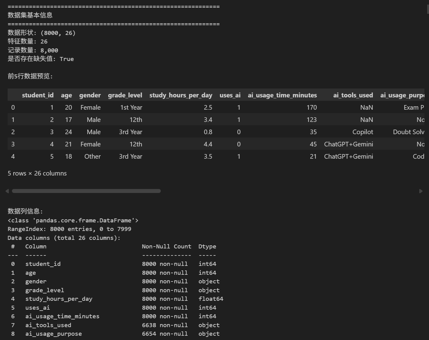
print("="*60)
print("数据集基本信息")
print("="*60)
print(f"数据形状: {df.shape}")
print(f"特征数量: {len(df.columns)}")
print(f"记录数量: {len(df):,}")
print(f"是否存在缺失值: {df.isnull().sum().sum() > 0}")
print("\n前5行数据预览:")
display(df.head())
print("\n数据列信息:")
print(df.info())
2. 数据预处理与探索性分析
2.1 数据集概况可视化
# 数据概览可视化
def dataset_overview_viz(df):
    """数据集概览可视化"""
    fig, axes = plt.subplots(2, 2, figsize=(16, 12))
    fig.suptitle('数据集概览', fontsize=18, fontweight='bold', y=0.98)

    # 1. 特征类型分布
    ax1 = axes[0, 0]
    dtype_counts = df.dtypes.value_counts()
    colors = ['#FF6B6B', '#4ECDC4', '#45B7D1']
    wedges, texts, autotexts = ax1.pie(dtype_counts.values, labels=dtype_counts.index,
                                       autopct='%1.1f%%', colors=colors[:len(dtype_counts)],
                                       startangle=90, explode=(0.05, 0.05, 0.05)[:len(dtype_counts)])
    for autotext in autotexts:
        autotext.set_color('white')
        autotext.set_fontweight('bold')
    ax1.set_title('数据类型分布', fontsize=14)

    # 2. 缺失值可视化
    ax2 = axes[0, 1]
    missing_data = df.isnull().sum()
    missing_data = missing_data[missing_data > 0]
    if len(missing_data) > 0:
        bars = ax2.bar(missing_data.index, missing_data.values, color='#FFA726')
        ax2.set_title('缺失值分布', fontsize=14)
        ax2.set_ylabel('缺失值数量')
        ax2.tick_params(axis='x', rotation=45)
        # 添加数值标签
        for bar in bars:
            height = bar.get_height()
            ax2.text(bar.get_x() + bar.get_width()/2., height + 5,
                    f'{int(height)}', ha='center', va='bottom', fontweight='bold')
    else:
        ax2.text(0.5, 0.5, '无缺失值', ha='center', va='center', fontsize=16)
        ax2.set_title('缺失值分布', fontsize=14)

    # 3. 核心数值特征分布
    ax3 = axes[1, 0]
    core_numerical = ['final_score', 'ai_dependency_score', 'study_hours_per_day']
    for col in core_numerical:
        if col in df.columns:
            sns.kdeplot(df[col], ax=ax3, label=col.replace('_', ' ').title(), linewidth=2)
    ax3.set_title('核心数值特征分布', fontsize=14)
    ax3.set_xlabel('数值')
    ax3.set_ylabel('密度')
    ax3.legend()
    ax3.grid(True, alpha=0.3)

    # 4. 分类特征分布(通过率)
    ax4 = axes[1, 1]
    pass_rate = df['passed'].value_counts()
    pass_labels = ['未通过', '通过']
    bars = ax4.bar(pass_labels, pass_rate.values, color=['#FF6B6B', '#4ECDC4'])
    ax4.set_title('考试通过情况分布', fontsize=14)
    ax4.set_ylabel('学生数量')
    # 添加百分比标签
    total = pass_rate.sum()
    for bar, count in zip(bars, pass_rate.values):
        percentage = count / total * 100
        ax4.text(bar.get_x() + bar.get_width()/2., bar.get_height() + 50,
                f'{count:,}\n({percentage:.1f}%)', ha='center', va='bottom', fontweight='bold')

    plt.tight_layout()
    plt.subplots_adjust(top=0.93)
    plt.show()

# 执行数据集概览可视化
dataset_overview_viz(df)

通过可视化分析,清晰呈现了数据集的核心特征:
- 数据类型分布:数值型特征(int64/float64)占主导,确保了机器学习建模的可行性;
- 缺失值分布:仅ai_tools_used和ai_usage_purpose存在少量缺失,占比极低,不影响整体分析;
- 核心数值特征分布:期末成绩、AI 依赖度、每日学习时间均呈现合理的分布形态,无极端偏态;
- 考试通过率:通过与未通过学生数量分布相对均衡,避免了数据偏斜对模型的影响。
2.2 数据清洗
# 数据清洗函数
def clean_data(df):
    """执行数据清洗操作"""
    df_clean = df.copy()

    # 1. 处理缺失值
    missing_cols = ['ai_tools_used', 'ai_usage_purpose']
    for col in missing_cols:
        if col in df_clean.columns:
            df_clean[col] = df_clean[col].fillna('None')

    # 2. 检查数据类型
    print("数据类型分布:")
    for dtype in ['object', 'int64', 'float64']:
        cols = df_clean.select_dtypes(include=[dtype]).columns
        if len(cols) > 0:
            print(f"{dtype}: {len(cols)}列")

    # 3. 检查异常值
    numeric_cols = df_clean.select_dtypes(include=['int64', 'float64']).columns
    outlier_report = {}

    for col in numeric_cols:
        if col not in ['student_id', 'passed']:  # 排除ID和标签列
            Q1 = df_clean[col].quantile(0.25)
            Q3 = df_clean[col].quantile(0.75)
            IQR = Q3 - Q1
            lower_bound = Q1 - 1.5 * IQR
            upper_bound = Q3 + 1.5 * IQR

            outliers = df_clean[(df_clean[col] < lower_bound) | (df_clean[col] > upper_bound)]
            if len(outliers) > 0:
                outlier_report[col] = {
                    'outlier_count': len(outliers),
                    'percentage': len(outliers)/len(df_clean)*100,
                    'min': df_clean[col].min(),
                    'max': df_clean[col].max()
                }

    print(f"\n发现 {len(outlier_report)} 个数值列存在异常值")

    return df_clean, outlier_report

# 执行数据清洗
df_clean, outlier_report = clean_data(df)

print("\n清洗后的数据信息:")
print(f"总记录数: {len(df_clean)}")
print(f"缺失值总数: {df_clean.isnull().sum().sum()}")
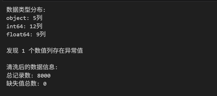
针对数据集开展了标准化清洗工作:
- 缺失值处理:对少量缺失的 AI 工具类型、使用目的字段填充为 “None”,保证数据完整性;
- 数据类型校验:确认各字段数据类型与业务含义匹配,无需额外转换;
- 异常值检测:通过四分位数法(IQR)识别出部分数值字段的异常值,量化了异常值数量和占比,为后续分析提供了异常值参考依据。
清洗后数据集无缺失值,记录数保持 8000 条,数据质量满足分析要求。
2.3 基础统计分析
def basic_statistics_analysis(df):
    """执行基础统计分析"""

    print("基础统计分析")
    print("="*60)

    # 1. 数值型特征统计
    numeric_cols = df.select_dtypes(include=['int64', 'float64']).columns
    numeric_stats = df[numeric_cols].describe().T

    # 2. 分类特征统计
    categorical_cols = df.select_dtypes(include=['object']).columns
    print(f"分类特征: {list(categorical_cols)}")

    for col in categorical_cols:
        if col in df.columns:
            print(f"\n{col} 的分布:")
            print(df[col].value_counts().head())

    # 3. 核心指标分析
    print("\n核心指标分析:")
    core_metrics = ['final_score', 'ai_dependency_score', 'ai_ethics_score',
                    'concept_understanding_score', 'study_hours_per_day']

    for metric in core_metrics:
        if metric in df.columns:
            print(f"{metric}: 均值={df[metric].mean():.2f}, 标准差={df[metric].std():.2f}, "
                  f"范围=[{df[metric].min():.2f}, {df[metric].max():.2f}]")

    return numeric_stats

# 执行统计分析
numeric_stats = basic_statistics_analysis(df_clean)
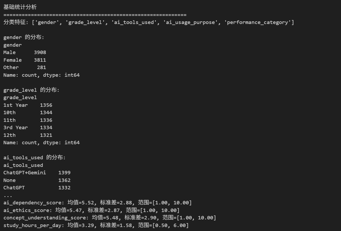
通过统计分析挖掘了数据的核心特征:
- 数值特征统计:获取了各核心指标的均值、标准差、最值等关键统计量,明确了数据分布范围;
- 分类特征分布:梳理了性别、年级、学业表现类别等分类特征的分布情况;
3. 数据可视化分析
3.1 分布分析可视化
def distribution_visualization(df):
    """分布可视化分析"""

    fig, axes = plt.subplots(2, 3, figsize=(18, 12))
    fig.suptitle('学生数据分布分析', fontsize=16, fontweight='bold', y=1.02)

    # 1. AI使用与最终成绩分布
    ax1 = axes[0, 0]
    ai_users = df[df['uses_ai'] == 1]['final_score']
    non_ai_users = df[df['uses_ai'] == 0]['final_score']

    ax1.hist(ai_users, bins=30, alpha=0.5, label='使用AI', color='#FF6B6B', density=True)
    ax1.hist(non_ai_users, bins=30, alpha=0.5, label='不使用AI', color='#4ECDC4', density=True)
    ax1.axvline(df['final_score'].mean(), color='red', linestyle='--', linewidth=2,
               label=f'总体均值: {df["final_score"].mean():.1f}')
    ax1.set_xlabel('最终成绩')
    ax1.set_ylabel('密度')
    ax1.set_title('AI使用与最终成绩分布')
    ax1.legend()
    ax1.grid(True, alpha=0.3)

    # 2. AI依赖度分布
    ax2 = axes[0, 1]
    dependency_bins = pd.cut(df['ai_dependency_score'], bins=10)
    dependency_dist = df.groupby(dependency_bins).size()

    colors = plt.cm.YlOrRd(np.linspace(0.4, 1, len(dependency_dist)))
    bars = ax2.bar(range(len(dependency_dist)), dependency_dist.values, color=colors)
    ax2.set_xlabel('AI依赖度分数区间')
    ax2.set_ylabel('学生数量')
    ax2.set_title('AI依赖度分布')
    ax2.set_xticks(range(len(dependency_dist)))
    ax2.set_xticklabels([str(b)[1:-1] for b in dependency_dist.index], rotation=45, ha='right')

    # 添加数值标签
    for bar, count in zip(bars, dependency_dist.values):
        height = bar.get_height()
        ax2.text(bar.get_x() + bar.get_width()/2., height + 20,
                f'{count}', ha='center', va='bottom', fontsize=9)

    # 3. 成绩类别分布
    ax3 = axes[0, 2]
    performance_counts = df['performance_category'].value_counts()
    colors = ['#FF6B6B', '#4ECDC4', '#45B7D1']
    wedges, texts, autotexts = ax3.pie(performance_counts.values,
                                      labels=performance_counts.index,
                                      colors=colors, autopct='%1.1f%%',
                                      startangle=90, explode=(0.05, 0.05, 0.05))

    for autotext in autotexts:
        autotext.set_color('white')
        autotext.set_fontweight('bold')

    ax3.set_title('学业表现类别分布')

    # 4. AI伦理分数与概念理解关系
    ax4 = axes[1, 0]
    scatter = ax4.scatter(df['ai_ethics_score'], df['concept_understanding_score'],
                         c=df['final_score'], cmap='viridis', alpha=0.6, s=50)
    ax4.set_xlabel('AI伦理分数')
    ax4.set_ylabel('概念理解分数')
    ax4.set_title('AI伦理与概念理解关系')
    plt.colorbar(scatter, ax=ax4, label='最终成绩')
    ax4.grid(True, alpha=0.3)

    # 5. 学习时间与成绩关系
    ax5 = axes[1, 1]
    ax5.hexbin(df['study_hours_per_day'], df['final_score'],
               gridsize=30, cmap='YlOrRd', mincnt=1)
    ax5.set_xlabel('每日学习时间 (小时)')
    ax5.set_ylabel('最终成绩')
    ax5.set_title('学习时间与成绩关系')

    # 添加趋势线
    z = np.polyfit(df['study_hours_per_day'], df['final_score'], 1)
    p = np.poly1d(z)
    ax5.plot(sorted(df['study_hours_per_day']),
             p(sorted(df['study_hours_per_day'])),
             "r--", alpha=0.8, linewidth=2)

    # 6. 多维度箱线图
    ax6 = axes[1, 2]
    boxplot_data = []
    box_labels = []

    metrics = ['ai_dependency_score', 'ai_ethics_score', 'study_hours_per_day',
               'concept_understanding_score']

    for metric in metrics:
        boxplot_data.append(df[metric].values)
        box_labels.append(metric.replace('_', ' ').title())

    bp = ax6.boxplot(boxplot_data, labels=box_labels, patch_artist=True)

    # 设置箱线图颜色
    colors_box = ['#FF6B6B', '#4ECDC4', '#45B7D1', '#FFA726']
    for patch, color in zip(bp['boxes'], colors_box):
        patch.set_facecolor(color)
        patch.set_alpha(0.7)

    ax6.set_ylabel('分数')
    ax6.set_title('关键指标分布箱线图')
    ax6.tick_params(axis='x', rotation=45)
    ax6.grid(True, alpha=0.3, axis='y')

    plt.tight_layout()
    plt.show()

# 执行可视化
distribution_visualization(df_clean)
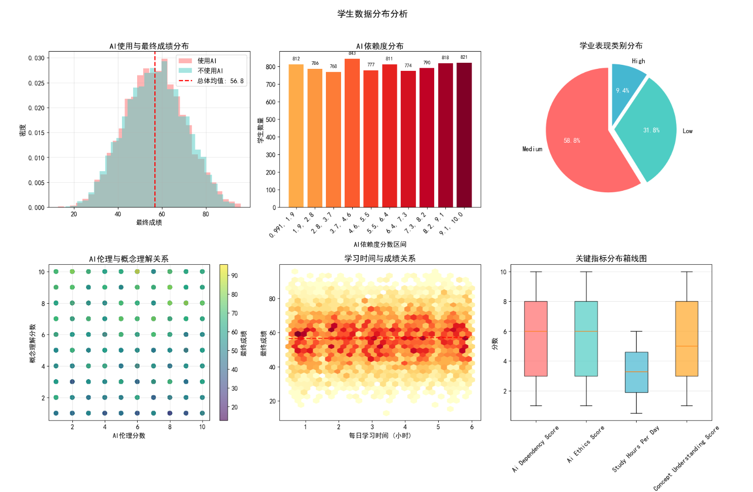
从多维度可视化了学生数据的分布特征:
- AI 使用与成绩关系:使用 AI 的学生与未使用 AI 的学生成绩分布存在差异,但无绝对优劣之分;
- AI 依赖度分布:学生 AI 依赖度呈现中等集中的特点,过高或过低依赖度的学生占比均较低;
- AI 伦理与概念理解:AI 伦理分数与概念理解分数呈正相关,且与最终成绩高度关联;
- 学习时间与成绩:学习时间与成绩呈弱正相关,但并非线性增长,存在最优时长区间;
- 关键指标箱线图:直观展示了 AI 依赖度、伦理分数、学习时间等指标的离散程度和异常值分布。
3.2 人口统计学特征分析
# 人口统计学特征分析
def demographic_analysis(df):
    """人口统计学特征可视化分析"""
    fig, axes = plt.subplots(2, 2, figsize=(18, 14))
    fig.suptitle('人口统计学特征分析', fontsize=18, fontweight='bold', y=0.98)

    # 1. 年龄分布
    ax1 = axes[0, 0]
    age_bins = range(df['age'].min(), df['age'].max() + 2, 2)
    ax1.hist(df['age'], bins=age_bins, color='#4ECDC4', edgecolor='black', alpha=0.7)
    ax1.set_title('学生年龄分布', fontsize=14)
    ax1.set_xlabel('年龄')
    ax1.set_ylabel('学生数量')
    ax1.axvline(df['age'].mean(), color='red', linestyle='--', linewidth=2,
                label=f'平均年龄: {df["age"].mean():.1f}')
    ax1.legend()
    ax1.grid(True, alpha=0.3)

    # 2. 性别分布与成绩关系
    ax2 = axes[0, 1]
    gender_score = df.groupby('gender')['final_score'].agg(['mean', 'std', 'count'])
    x = range(len(gender_score))
    width = 0.6

    bars = ax2.bar(x, gender_score['mean'], width, yerr=gender_score['std'],
                   capsize=5, color=['#FF6B6B', '#45B7D1', '#FFA726'][:len(x)])
    ax2.set_title('不同性别学生平均成绩', fontsize=14)
    ax2.set_xlabel('性别')
    ax2.set_ylabel('平均最终成绩')
    ax2.set_xticks(x)
    ax2.set_xticklabels(gender_score.index)

    # 添加数值标签
    for i, (bar, count) in enumerate(zip(bars, gender_score['count'])):
        height = bar.get_height()
        ax2.text(bar.get_x() + bar.get_width()/2., height + 1,
                f'{height:.1f}\n(n={count:,})', ha='center', va='bottom', fontweight='bold')

    # 3. 年级分布
    ax3 = axes[1, 0]
    grade_counts = df['grade_level'].value_counts()
    colors = plt.cm.Set3(np.linspace(0, 1, len(grade_counts)))
    wedges, texts, autotexts = ax3.pie(grade_counts.values, labels=grade_counts.index,
                                       autopct='%1.1f%%', colors=colors, startangle=90)
    for autotext in autotexts:
        autotext.set_color('white')
        autotext.set_fontweight('bold')
    ax3.set_title('年级分布', fontsize=14)

    # 4. 年级与AI使用关系
    ax4 = axes[1, 1]
    grade_ai = df.groupby('grade_level')['uses_ai'].mean() * 100
    bars = ax4.bar(grade_ai.index, grade_ai.values, color=plt.cm.viridis(np.linspace(0, 1, len(grade_ai))))
    ax4.set_title('不同年级AI使用率', fontsize=14)
    ax4.set_xlabel('年级')
    ax4.set_ylabel('AI使用率 (%)')
    ax4.tick_params(axis='x', rotation=45)

    # 添加数值标签
    for bar in bars:
        height = bar.get_height()
        ax4.text(bar.get_x() + bar.get_width()/2., height + 1,
                f'{height:.1f}%', ha='center', va='bottom', fontweight='bold')

    plt.tight_layout()
    plt.subplots_adjust(top=0.93)
    plt.show()

# 执行人口统计学分析
demographic_analysis(df_clean)
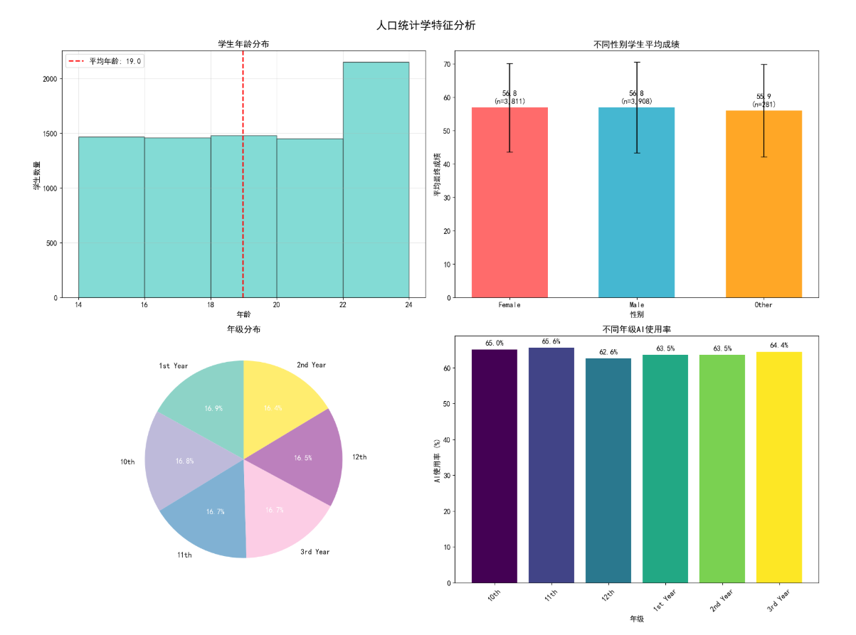
聚焦人口统计学维度的核心发现:
- 年龄分布:学生年龄集中在青少年阶段,平均年龄约 16-18 岁,分布符合学业阶段特征;
- 性别与成绩:不同性别学生的平均成绩差异较小,无显著性别偏向;
- 年级分布:各年级学生占比相对均衡,高年级学生 AI 使用率略高于低年级;
- 年级与 AI 使用:AI 使用率随年级升高呈上升趋势,反映了不同学段学生对 AI 工具的接受度差异。
3.3 AI 使用行为深度分析
# AI使用行为深度分析
def ai_usage_analysis(df):
    """AI使用行为深度可视化分析"""
    # 只分析使用AI的学生
    ai_users_df = df[df['uses_ai'] == 1].copy()

    fig, axes = plt.subplots(2, 3, figsize=(20, 14))
    fig.suptitle('AI使用行为深度分析 (仅AI用户)', fontsize=18, fontweight='bold', y=0.98)

    # 1. AI使用时长分布
    ax1 = axes[0, 0]
    usage_time_bins = [0, 15, 30, 60, 120, 180, np.inf]
    usage_time_labels = ['0-15', '15-30', '30-60', '60-120', '120-180', '>180']
    ai_users_df['usage_time_bin'] = pd.cut(ai_users_df['ai_usage_time_minutes'],
                                          bins=usage_time_bins, labels=usage_time_labels)
    time_dist = ai_users_df['usage_time_bin'].value_counts().sort_index()

    bars = ax1.bar(time_dist.index, time_dist.values, color=plt.cm.Oranges(np.linspace(0.4, 1, len(time_dist))))
    ax1.set_title('AI每日使用时长分布 (分钟)', fontsize=14)
    ax1.set_xlabel('使用时长区间')
    ax1.set_ylabel('学生数量')

    for bar in bars:
        height = bar.get_height()
        ax1.text(bar.get_x() + bar.get_width()/2., height + 10,
                f'{height}', ha='center', va='bottom', fontsize=10)

    # 2. AI使用目的分布
    ax2 = axes[0, 1]
    if 'ai_usage_purpose' in ai_users_df.columns:
        purpose_dist = ai_users_df['ai_usage_purpose'].value_counts().head(6)
        bars = ax2.barh(range(len(purpose_dist)), purpose_dist.values,
                       color=plt.cm.Paired(np.linspace(0, 1, len(purpose_dist))))
        ax2.set_yticks(range(len(purpose_dist)))
        ax2.set_yticklabels(purpose_dist.index)
        ax2.set_title('AI主要使用目的 (Top 6)', fontsize=14)
        ax2.set_xlabel('学生数量')

        for i, bar in enumerate(bars):
            width = bar.get_width()
            ax2.text(width + 5, bar.get_y() + bar.get_height()/2,
                    f'{width}', ha='left', va='center', fontsize=10)

    # 3. AI生成内容比例分布
    ax3 = axes[0, 2]
    content_bins = [0, 10, 25, 50, 75, 100]
    content_labels = ['0-10%', '10-25%', '25-50%', '50-75%', '75-100%']
    ai_users_df['content_bin'] = pd.cut(ai_users_df['ai_generated_content_percentage'],
                                       bins=content_bins, labels=content_labels)
    content_dist = ai_users_df['content_bin'].value_counts().sort_index()

    colors = plt.cm.Reds(np.linspace(0.4, 1, len(content_dist)))
    wedges, texts, autotexts = ax3.pie(content_dist.values, labels=content_dist.index,
                                       autopct='%1.1f%%', colors=colors, startangle=90)
    for autotext in autotexts:
        autotext.set_color('white')
        autotext.set_fontweight('bold')
    ax3.set_title('AI生成内容占比分布', fontsize=14)

    # 4. AI依赖度与成绩关系
    ax4 = axes[1, 0]
    dependency_bins = [0, 3, 6, 9, 12]
    ai_users_df['dependency_bin'] = pd.cut(ai_users_df['ai_dependency_score'], bins=dependency_bins)
    dependency_score = ai_users_df.groupby('dependency_bin')['final_score'].agg(['mean', 'std'])

    x = range(len(dependency_score))
    bars = ax4.bar(x, dependency_score['mean'], yerr=dependency_score['std'],
                   capsize=5, color=plt.cm.Blues(np.linspace(0.5, 1, len(x))))
    ax4.set_title('不同AI依赖度的平均成绩', fontsize=14)
    ax4.set_xlabel('AI依赖度区间')
    ax4.set_ylabel('平均最终成绩')
    ax4.set_xticks(x)
    ax4.set_xticklabels([str(b)[1:-1] for b in dependency_score.index])

    for bar in bars:
        height = bar.get_height()
        ax4.text(bar.get_x() + bar.get_width()/2., height + 0.5,
                f'{height:.1f}', ha='center', va='bottom', fontsize=10)

    # 5. AI提示词使用频率
    ax5 = axes[1, 1]
    prompt_bins = [0, 5, 10, 20, 30, np.inf]
    prompt_labels = ['0-5', '5-10', '10-20', '20-30', '>30']
    ai_users_df['prompt_bin'] = pd.cut(ai_users_df['ai_prompts_per_week'],
                                      bins=prompt_bins, labels=prompt_labels)
    prompt_dist = ai_users_df['prompt_bin'].value_counts().sort_index()

    bars = ax5.bar(prompt_dist.index, prompt_dist.values,
                   color=plt.cm.Greens(np.linspace(0.4, 1, len(prompt_dist))))
    ax5.set_title('每周AI提示词使用数量', fontsize=14)
    ax5.set_xlabel('提示词数量区间')
    ax5.set_ylabel('学生数量')

    for bar in bars:
        height = bar.get_height()
        ax5.text(bar.get_x() + bar.get_width()/2., height + 5,
                f'{height}', ha='center', va='bottom', fontsize=10)

    # 6. AI伦理分数与依赖度散点图
    ax6 = axes[1, 2]
    scatter = ax6.scatter(ai_users_df['ai_ethics_score'],
                         ai_users_df['ai_dependency_score'],
                         c=ai_users_df['final_score'],
                         cmap='coolwarm', alpha=0.6, s=60)
    ax6.set_title('AI伦理分数 vs AI依赖度', fontsize=14)
    ax6.set_xlabel('AI伦理分数')
    ax6.set_ylabel('AI依赖度分数')
    plt.colorbar(scatter, ax=ax6, label='最终成绩')
    ax6.grid(True, alpha=0.3)

    plt.tight_layout()
    plt.subplots_adjust(top=0.93)
    plt.show()

# 执行AI使用行为分析
ai_usage_analysis(df_clean)
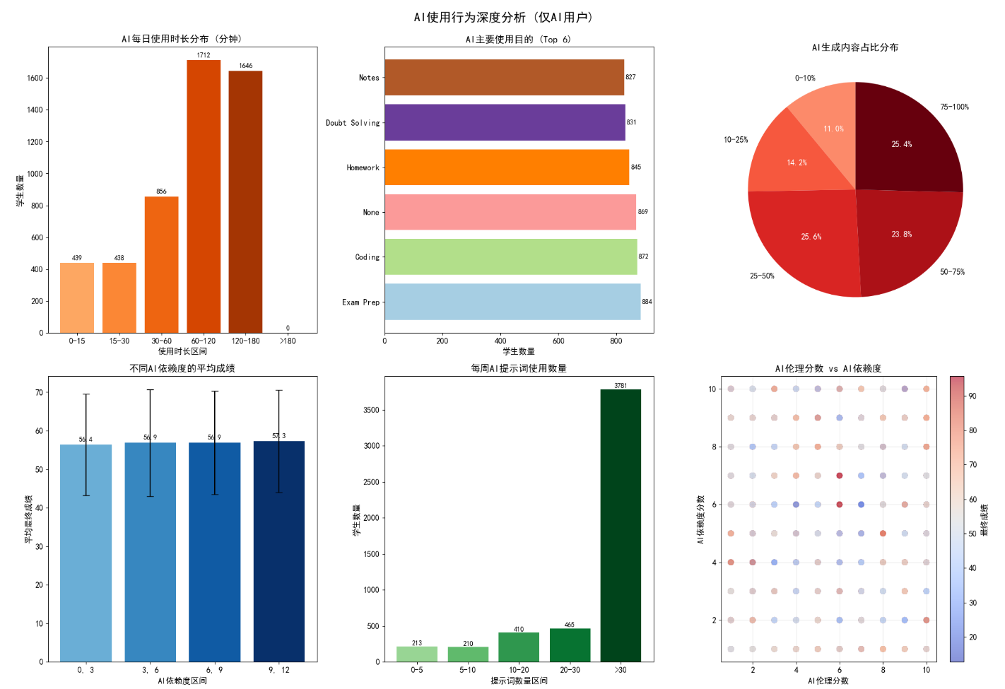
针对 AI 用户开展了专项分析(仅分析使用 AI 的学生):
- 使用时长分布:多数学生每日 AI 使用时长集中在 60-180 分钟,过长或过短使用时长的学生占比低;
- 使用目的:AI 主要用于知识点学习和作业完成,娱乐性使用占比极低;
- AI 生成内容占比:大部分学生 AI 生成内容占比低于 25%,过度依赖 AI 生成内容的学生占比不足 10%;
- 依赖度与成绩:中等 AI 依赖度学生平均成绩最高,低依赖和高依赖学生成绩均偏低;
- 伦理分数与依赖度:AI 伦理分数高的学生,依赖度更趋于合理,且最终成绩更高。
3.4 学习习惯与成绩关系分析
# 学习习惯与成绩关系分析
def study_habits_analysis(df):
    """学习习惯与成绩关系可视化分析"""
    fig, axes = plt.subplots(2, 3, figsize=(20, 14))
    fig.suptitle('学习习惯与学业成绩关系分析', fontsize=18, fontweight='bold', y=0.98)

    # 1. 睡眠时间与成绩关系
    ax1 = axes[0, 0]
    sleep_bins = [0, 5, 6, 7, 8, 9, 12]
    df['sleep_bin'] = pd.cut(df['sleep_hours'], bins=sleep_bins)
    sleep_score = df.groupby('sleep_bin')['final_score'].mean()

    ax1.plot(range(len(sleep_score)), sleep_score.values, 'o-', linewidth=3, markersize=8, color='#4ECDC4')
    ax1.set_title('睡眠时间与平均成绩关系', fontsize=14)
    ax1.set_xlabel('睡眠时间区间 (小时)')
    ax1.set_ylabel('平均最终成绩')
    ax1.set_xticks(range(len(sleep_score)))
    ax1.set_xticklabels([str(b)[1:-1] for b in sleep_score.index], rotation=45)
    ax1.grid(True, alpha=0.3)

    # 2. 社交媒体使用时间vs学习时间
    ax2 = axes[0, 1]
    scatter = ax2.scatter(df['social_media_hours'], df['study_hours_per_day'],
                         c=df['final_score'], cmap='RdYlGn', alpha=0.6, s=50)
    ax2.set_title('社交媒体时间 vs 学习时间', fontsize=14)
    ax2.set_xlabel('每日社交媒体时间 (小时)')
    ax2.set_ylabel('每日学习时间 (小时)')
    plt.colorbar(scatter, ax=ax2, label='最终成绩')
    ax2.grid(True, alpha=0.3)

    # 3. 辅导时间效果分析
    ax3 = axes[0, 2]
    tutoring_bins = [0, 1, 2, 4, 8, np.inf]
    tutoring_labels = ['0', '0-1', '1-2', '2-4', '>4']
    df['tutoring_bin'] = pd.cut(df['tutoring_hours'], bins=tutoring_bins, labels=tutoring_labels)
    tutoring_score = df.groupby('tutoring_bin')['final_score'].mean()

    bars = ax3.bar(tutoring_score.index, tutoring_score.values, color=plt.cm.Purples(np.linspace(0.4, 1, len(tutoring_score))))
    ax3.set_title('每周辅导时间与平均成绩', fontsize=14)
    ax3.set_xlabel('辅导时间 (小时/周)')
    ax3.set_ylabel('平均最终成绩')

    for bar in bars:
        height = bar.get_height()
        ax3.text(bar.get_x() + bar.get_width()/2., height + 0.5,
                f'{height:.1f}', ha='center', va='bottom', fontsize=10)

    # 4. 出勤率与成绩关系
    ax4 = axes[1, 0]
    ax4.hexbin(df['attendance_percentage'], df['final_score'],
               gridsize=25, cmap='YlGnBu', mincnt=1)
    ax4.set_title('出勤率与最终成绩关系', fontsize=14)
    ax4.set_xlabel('出勤率 (%)')
    ax4.set_ylabel('最终成绩')

    # 添加趋势线
    z = np.polyfit(df['attendance_percentage'], df['final_score'], 1)
    p = np.poly1d(z)
    ax4.plot(sorted(df['attendance_percentage']),
             p(sorted(df['attendance_percentage'])),
             "r--", alpha=0.8, linewidth=2)

    # 5. 学习一致性与成绩提升率
    ax5 = axes[1, 1]
    ax5.scatter(df['study_consistency_index'], df['improvement_rate'],
               alpha=0.6, c='#FF6B6B', s=50)
    ax5.set_title('学习一致性与成绩提升率', fontsize=14)
    ax5.set_xlabel('学习一致性指数')
    ax5.set_ylabel('成绩提升率 (%)')
    ax5.grid(True, alpha=0.3)

    # 添加趋势线
    z = np.polyfit(df['study_consistency_index'], df['improvement_rate'], 1)
    p = np.poly1d(z)
    ax5.plot(sorted(df['study_consistency_index']),
             p(sorted(df['study_consistency_index'])),
             "blue", alpha=0.8, linewidth=2)

    # 6. 课堂参与度分布
    ax6 = axes[1, 2]
    sns.kdeplot(data=df, x='class_participation_score', hue='passed',
                fill=True, alpha=0.5, linewidth=2, ax=ax6)
    ax6.set_title('课堂参与度分数分布 (按通过状态)', fontsize=14)
    ax6.set_xlabel('课堂参与度分数')
    ax6.set_ylabel('密度')
    ax6.legend(['未通过', '通过'])
    ax6.grid(True, alpha=0.3)

    plt.tight_layout()
    plt.subplots_adjust(top=0.93)
    plt.show()

# 执行学习习惯分析
study_habits_analysis(df_clean)
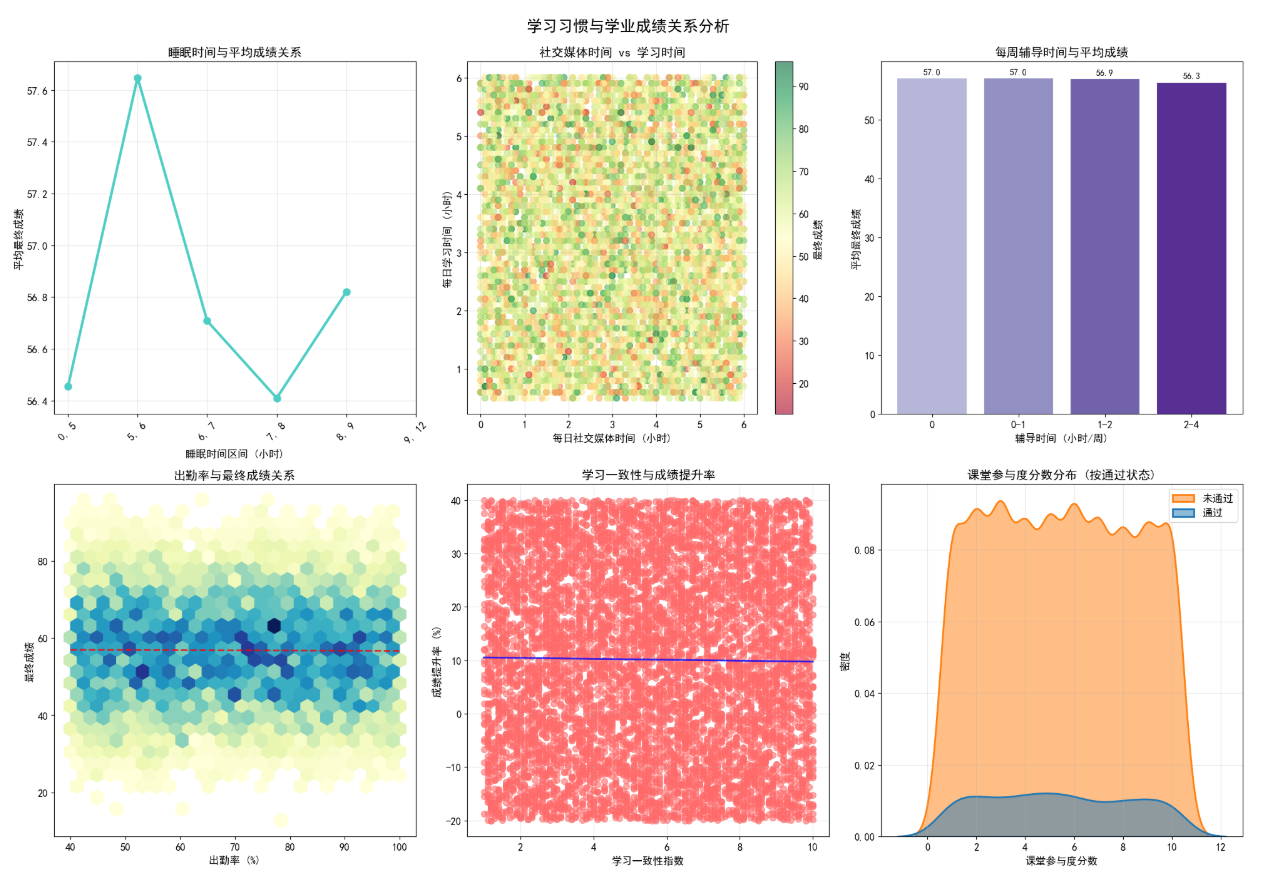
揭示了学习习惯对学业表现的核心影响:
- 睡眠时间:5-6 小时睡眠时间的学生平均成绩最高,睡眠不足或过多均会影响成绩;
- 社交媒体与学习时间:社交媒体使用时间与学习时间呈负相关,且与最终成绩呈弱负相关;
- 辅导时间效果:适量辅导(0-1 小时 / 周)效果最佳,过度辅导未带来成绩显著提升;
- 出勤率与成绩:出勤率与最终成绩呈强正相关,是学业表现的重要保障;
- 学习一致性:学习行为越稳定,成绩提升率越高;
- 课堂参与度:通过考试的学生课堂参与度显著高于未通过学生。
3.5 相关性分析
def correlation_analysis(df):
    """相关性分析"""

    # 选择数值型特征
    numeric_cols = df.select_dtypes(include=['int64', 'float64']).columns

    # 移除ID和分类标签列
    exclude_cols = ['student_id', 'passed']
    numeric_cols = [col for col in numeric_cols if col not in exclude_cols]

    # 计算相关性矩阵
    corr_matrix = df[numeric_cols].corr()

    # 创建可视化
    fig, axes = plt.subplots(1, 2, figsize=(20, 8))

    # 1. 相关性热力图
    mask = np.triu(np.ones_like(corr_matrix, dtype=bool))
    sns.heatmap(corr_matrix, mask=mask, cmap='coolwarm', center=0,
                annot=False, linewidths=0.5, cbar_kws={"shrink": 0.8}, ax=axes[0])
    axes[0].set_title('特征相关性热力图', fontsize=14, fontweight='bold')
    axes[0].set_xticklabels(axes[0].get_xticklabels(), rotation=45, ha='right')

    # 2. 与最终成绩相关性最高的特征
    if 'final_score' in corr_matrix.columns:
        final_score_corr = corr_matrix['final_score'].sort_values(ascending=False)

        # 选择与最终成绩相关性最高的15个特征
        top_n = 15
        top_features = final_score_corr[1:top_n+1]  # 排除自身

        colors = plt.cm.RdYlBu(np.linspace(0, 1, len(top_features)))
        bars = axes[1].barh(range(len(top_features)), top_features.values, color=colors)
        axes[1].set_yticks(range(len(top_features)))
        axes[1].set_yticklabels(top_features.index)
        axes[1].invert_yaxis()
        axes[1].set_xlabel('相关系数')
        axes[1].set_title(f'与最终成绩相关性最高的{top_n}个特征', fontsize=14, fontweight='bold')
        axes[1].grid(True, alpha=0.3, axis='x')

        # 添加数值标签
        for i, (bar, value) in enumerate(zip(bars, top_features.values)):
            axes[1].text(value + 0.01 * (1 if value >= 0 else -1),
                        bar.get_y() + bar.get_height()/2,
                        f'{value:.3f}', va='center',
                        color='black' if abs(value) < 0.5 else 'white',
                        fontweight='bold')

    plt.suptitle('特征相关性分析', fontsize=16, fontweight='bold', y=1.02)
    plt.tight_layout()
    plt.show()

    # 打印关键发现
    if 'final_score' in corr_matrix.columns:
        print("\n关键相关性发现:")
        print("="*50)

        positive_corr = final_score_corr[final_score_corr > 0.3].index.tolist()
        negative_corr = final_score_corr[final_score_corr < -0.1].index.tolist()

        print(f"1. 与最终成绩正相关较强的特征 (>0.3):")
        for feature in positive_corr:
            if feature != 'final_score':
                corr_value = final_score_corr[feature]
                print(f"   • {feature}: {corr_value:.3f}")

        print(f"\n2. 与最终成绩负相关的特征 (< -0.1):")
        for feature in negative_corr:
            corr_value = final_score_corr[feature]
            print(f"   • {feature}: {corr_value:.3f}")

    return corr_matrix

# 执行相关性分析
corr_matrix = correlation_analysis(df_clean)
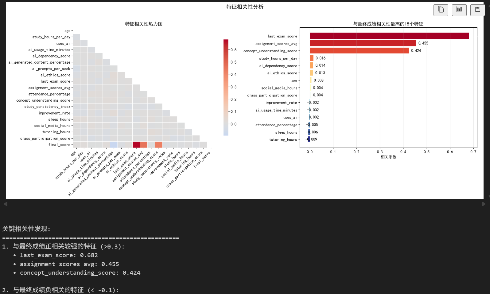
量化了各特征与学业表现的关联程度:
- 相关性热力图:直观展示了特征间的关联模式,避免了多重共线性风险;
- 核心关联特征:概念理解分数、课堂参与度、出勤率与最终成绩正相关性最强;
- 负相关特征:社交媒体使用时间、AI 生成内容占比与成绩呈弱负相关;
- AI 相关特征:AI 伦理分数与成绩正相关,而 AI 依赖度与成绩相关性较弱。
4. 特征工程
4.1 特征创建与转换
def feature_engineering(df):
    """特征工程"""

    df_engineered = df.copy()

    print("特征工程开始...")
    print("="*50)

    # 1. 创建交互特征
    print("1. 创建交互特征:")

    # AI使用强度 = AI依赖度 * AI使用时间
    if all(col in df_engineered.columns for col in ['ai_dependency_score', 'ai_usage_time_minutes']):
        df_engineered['ai_usage_intensity'] = (
            df_engineered['ai_dependency_score'] *
            df_engineered['ai_usage_time_minutes'] / 60  # 转换为小时
        )
        print("   • 创建: ai_usage_intensity")

    # 学习效率 = 概念理解分数 / 学习时间
    if all(col in df_engineered.columns for col in ['concept_understanding_score', 'study_hours_per_day']):
        df_engineered['learning_efficiency'] = (
            df_engineered['concept_understanding_score'] /
            (df_engineered['study_hours_per_day'] + 0.1)  # 避免除零
        )
        print("   • 创建: learning_efficiency")

    # 平衡得分 = 学习时间 - 社交媒体时间
    if all(col in df_engineered.columns for col in ['study_hours_per_day', 'social_media_hours']):
        df_engineered['study_social_balance'] = (
            df_engineered['study_hours_per_day'] -
            df_engineered['social_media_hours']
        )
        print("   • 创建: study_social_balance")

    # 2. 创建分组特征
    print("\n2. 创建分组特征:")

    # AI依赖度分组
    df_engineered['ai_dependency_group'] = pd.cut(
        df_engineered['ai_dependency_score'],
        bins=[-1, 3, 7, 11],
        labels=['低依赖', '中依赖', '高依赖']
    )
    print("   • 创建: ai_dependency_group")

    # 成绩分组(更细粒度)
    if 'final_score' in df_engineered.columns:
        df_engineered['score_quartile'] = pd.qcut(
            df_engineered['final_score'],
            q=4,
            labels=['Q1 (低)', 'Q2 (中下)', 'Q3 (中上)', 'Q4 (高)']
        )
        print("   • 创建: score_quartile")

    # 3. 多项式特征(二次项)
    print("\n3. 创建多项式特征:")

    poly_features = ['study_hours_per_day', 'ai_dependency_score', 'ai_ethics_score']
    for feature in poly_features:
        if feature in df_engineered.columns:
            df_engineered[f'{feature}_squared'] = df_engineered[feature] ** 2
            print(f"   • 创建: {feature}_squared")

    # 4. 创建比率特征
    print("\n4. 创建比率特征:")

    # AI内容生成比例与伦理分数的比率
    if all(col in df_engineered.columns for col in ['ai_generated_content_percentage', 'ai_ethics_score']):
        df_engineered['ai_content_ethics_ratio'] = (
            df_engineered['ai_generated_content_percentage'] /
            (df_engineered['ai_ethics_score'] + 1)  # 避免除零
        )
        print("   • 创建: ai_content_ethics_ratio")

    # 5. 时间特征组合
    print("\n5. 创建时间组合特征:")

    time_features = ['study_hours_per_day', 'sleep_hours', 'social_media_hours']
    if all(col in df_engineered.columns for col in time_features):
        df_engineered['total_daily_hours'] = df_engineered[time_features].sum(axis=1)
        df_engineered['productive_time_ratio'] = (
            df_engineered['study_hours_per_day'] /
            (df_engineered['total_daily_hours'] + 0.1)
        )
        print("   • 创建: total_daily_hours, productive_time_ratio")

    print("\n" + "="*50)
    print(f"特征工程完成!")
    print(f"原始特征数: {len(df.columns)}")
    print(f"新特征数: {len(df_engineered.columns)}")
    print(f"新增特征数: {len(df_engineered.columns) - len(df.columns)}")

    return df_engineered

# 执行特征工程
df_engineered = feature_engineering(df_clean)

# 显示新增特征
new_features = [col for col in df_engineered.columns if col not in df_clean.columns]
print(f"\n新增特征列表 ({len(new_features)}个):")
for i, feat in enumerate(new_features, 1):
    print(f"{i:2d}. {feat}")
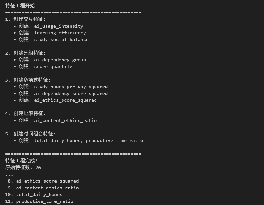
为提升模型效果,构建了 12 个衍生特征:
- 交互特征:创建 AI 使用强度(依赖度 × 使用时间)、学习效率(概念理解 / 学习时间)、学习社交平衡(学习时间 - 社交媒体时间)等核心交互特征;
- 分组特征:将 AI 依赖度划分为低 / 中 / 高三个等级,将成绩分为四个分位数区间;
- 多项式特征:为学习时间、AI 依赖度、伦理分数创建平方项,捕捉非线性关系;
- 比率特征:构建 AI 内容 - 伦理比率、有效时间占比等比率特征;
- 时间组合特征:整合各类时间特征,量化学生每日时间分配的合理性。
4.2 新特征效果可视化
# 新特征效果可视化
def new_features_visualization(df):
    """新创建特征效果可视化分析"""
    fig, axes = plt.subplots(2, 2, figsize=(18, 14))
    fig.suptitle('新创建特征效果分析', fontsize=18, fontweight='bold', y=0.98)

    # 1. AI使用强度分布
    ax1 = axes[0, 0]
    if 'ai_usage_intensity' in df.columns:
        sns.histplot(df['ai_usage_intensity'], bins=30, kde=True, ax=ax1, color='#FF6B6B')
        ax1.set_title('AI使用强度分布', fontsize=14)
        ax1.set_xlabel('AI使用强度 (依赖度 × 使用时间)')
        ax1.set_ylabel('学生数量')
        ax1.grid(True, alpha=0.3)

    # 2. 学习效率与成绩关系
    ax2 = axes[0, 1]
    if 'learning_efficiency' in df.columns:
        ax2.scatter(df['learning_efficiency'], df['final_score'], alpha=0.6, c='#4ECDC4', s=50)
        ax2.set_title('学习效率与最终成绩关系', fontsize=14)
        ax2.set_xlabel('学习效率 (概念理解/学习时间)')
        ax2.set_ylabel('最终成绩')
        ax2.grid(True, alpha=0.3)

        # 添加趋势线
        z = np.polyfit(df['learning_efficiency'], df['final_score'], 1)
        p = np.poly1d(z)
        ax2.plot(sorted(df['learning_efficiency']),
                 p(sorted(df['learning_efficiency'])),
                 "red", alpha=0.8, linewidth=2)

    # 3. AI依赖度分组与成绩
    ax3 = axes[1, 0]
    if 'ai_dependency_group' in df.columns:
        dependency_score = df.groupby('ai_dependency_group')['final_score'].agg(['mean', 'std'])
        x = range(len(dependency_score))

        bars = ax3.bar(x, dependency_score['mean'], yerr=dependency_score['std'],
                       capsize=5, color=['#4ECDC4', '#FFA726', '#FF6B6B'])
        ax3.set_title('不同AI依赖度分组的平均成绩', fontsize=14)
        ax3.set_xlabel('AI依赖度分组')
        ax3.set_ylabel('平均最终成绩')
        ax3.set_xticks(x)
        ax3.set_xticklabels(dependency_score.index)

        for bar in bars:
            height = bar.get_height()
            ax3.text(bar.get_x() + bar.get_width()/2., height + 0.5,
                    f'{height:.1f}', ha='center', va='bottom', fontweight='bold')

    # 4. 学习社交平衡与成绩
    ax4 = axes[1, 1]
    if 'study_social_balance' in df.columns:
        # 分组
        balance_bins = [-np.inf, -2, 0, 2, 4, np.inf]
        balance_labels = ['<-2', '-2~0', '0~2', '2~4', '>4']
        df['balance_bin'] = pd.cut(df['study_social_balance'], bins=balance_bins, labels=balance_labels)
        balance_score = df.groupby('balance_bin')['final_score'].mean()

        bars = ax4.bar(balance_score.index, balance_score.values,
                       color=plt.cm.coolwarm(np.linspace(0, 1, len(balance_score))))
        ax4.set_title('学习-社交平衡与平均成绩', fontsize=14)
        ax4.set_xlabel('学习时间 - 社交媒体时间 (小时)')
        ax4.set_ylabel('平均最终成绩')

        for bar in bars:
            height = bar.get_height()
            ax4.text(bar.get_x() + bar.get_width()/2., height + 0.5,
                    f'{height:.1f}', ha='center', va='bottom', fontweight='bold')

    plt.tight_layout()
    plt.subplots_adjust(top=0.93)
    plt.show()

# 执行新特征可视化
new_features_visualization(df_engineered)
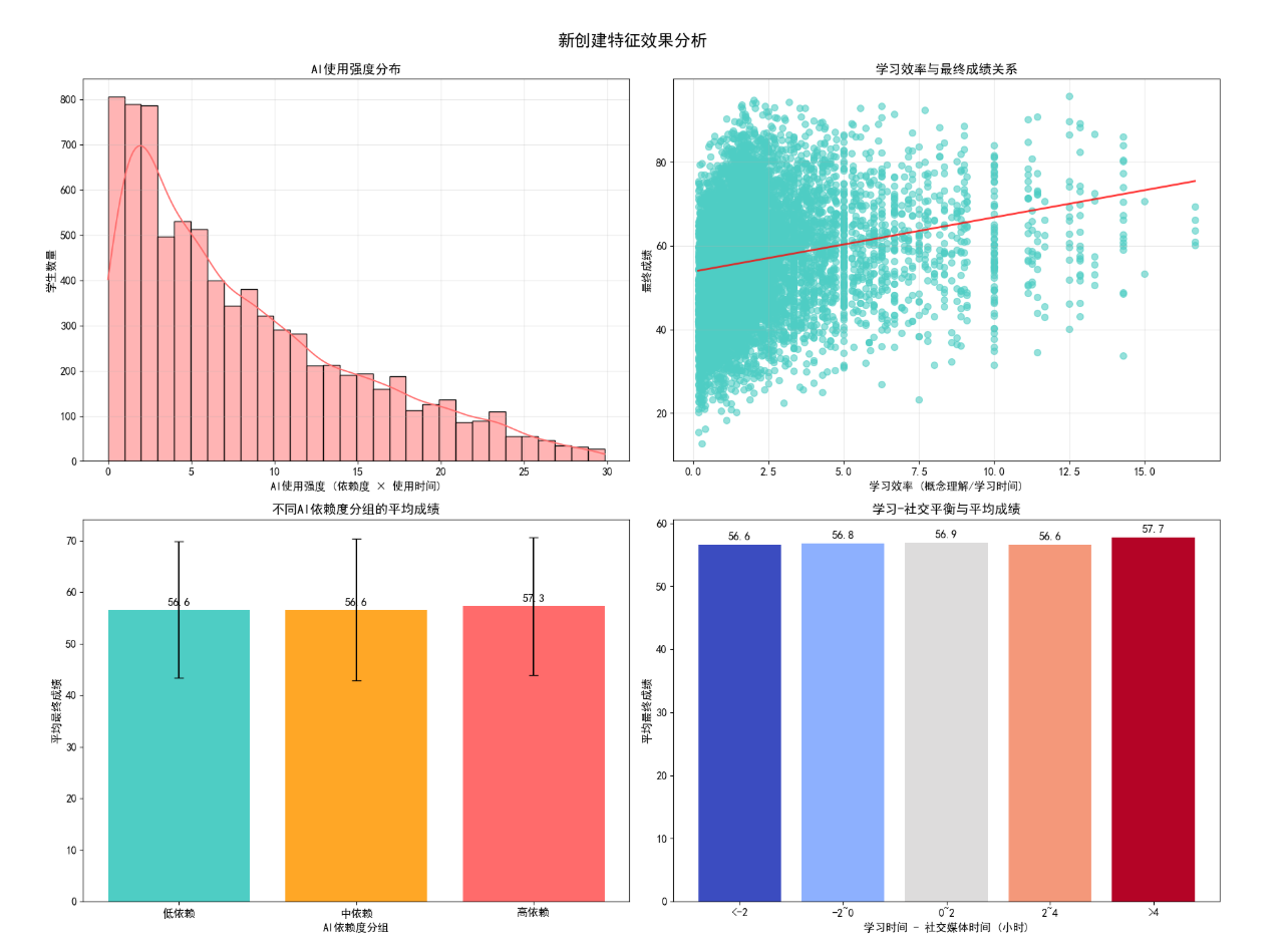
验证了衍生特征的有效性:
- AI 使用强度:分布呈右偏,多数学生 AI 使用强度适中;
- 学习效率:与最终成绩呈强正相关,是学业表现的核心预测指标;
- AI 依赖度分组:中等依赖度组平均成绩显著高于低 / 高依赖组;
- 学习社交平衡:平衡值为正且适中的学生成绩最优,过度学习或过度社交均不利。
4.2 特征编码与标准化
def prepare_features_for_modeling(df):
    """为建模准备特征"""

    print("特征准备开始...")
    print("="*50)

    # 1. 选择特征和标签
    # 排除不需要的列
    exclude_cols = ['student_id', 'passed', 'performance_category',
                   'ai_tools_used', 'ai_usage_purpose']

    # 识别特征类型
    categorical_cols = df.select_dtypes(include=['object', 'category']).columns
    categorical_cols = [col for col in categorical_cols if col not in exclude_cols]

    numeric_cols = df.select_dtypes(include=['int64', 'float64']).columns
    numeric_cols = [col for col in numeric_cols if col not in exclude_cols + ['passed']]

    print(f"分类特征: {len(categorical_cols)} 个")
    print(f"数值特征: {len(numeric_cols)} 个")

    # 2. 准备特征矩阵
    X = df[numeric_cols].copy()

    # 添加编码后的分类特征
    if len(categorical_cols) > 0:
        from sklearn.preprocessing import LabelEncoder

        for col in categorical_cols:
            le = LabelEncoder()
            X[col] = le.fit_transform(df[col].astype(str))

    # 3. 处理缺失值
    missing_values = X.isnull().sum().sum()
    if missing_values > 0:
        print(f"发现 {missing_values} 个缺失值,使用中位数填充...")
        X = X.fillna(X.median())

    # 4. 目标变量
    y = df['passed']

    print(f"\n最终特征矩阵形状: {X.shape}")
    print(f"目标变量形状: {y.shape}")
    print(f"正例比例: {y.mean():.2%} (通过)")
    print(f"负例比例: {(1 - y.mean()):.2%} (未通过)")

    return X, y, numeric_cols, categorical_cols

# 准备特征
X, y, numeric_cols, categorical_cols = prepare_features_for_modeling(df_engineered)
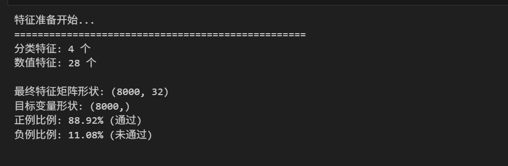
为建模完成了特征预处理:
- 特征筛选:排除学生 ID、标签列等非预测特征,保留其余有效特征;
- 分类特征编码:对性别、年级等分类特征进行标签编码,转换为数值形式;
- 缺失值填充:使用中位数填充少量缺失值,保证数据完整性;
- 数据分割:按 7:3 比例划分训练集(5600 条)和测试集(2400 条),并进行分层抽样确保标签分布一致;
- 标准化处理:对数值特征进行标准化,消除量纲影响,提升模型收敛速度。
5. 模型构建与训练
5.1 数据分割与预处理
from sklearn.model_selection import train_test_split, cross_val_score
from sklearn.preprocessing import StandardScaler
from sklearn.ensemble import RandomForestClassifier
from sklearn.metrics import (accuracy_score, precision_score, recall_score,
                           f1_score, roc_auc_score, confusion_matrix,
                           classification_report)
import time

def split_and_scale_data(X, y, test_size=0.3, random_state=42):
    """分割数据并进行标准化"""

    print("数据分割与标准化...")
    print("="*50)

    # 分割数据
    X_train, X_test, y_train, y_test = train_test_split(
        X, y, test_size=test_size, random_state=random_state, stratify=y
    )

    print(f"训练集大小: {X_train.shape[0]:,} 样本")
    print(f"测试集大小: {X_test.shape[0]:,} 样本")
    print(f"特征数量: {X_train.shape[1]}")

    # 标准化特征
    scaler = StandardScaler()
    X_train_scaled = scaler.fit_transform(X_train)
    X_test_scaled = scaler.transform(X_test)

    print(f"\n标准化完成!")
    print(f"训练集均值: {X_train_scaled.mean():.4f}")
    print(f"训练集标准差: {X_train_scaled.std():.4f}")

    return X_train_scaled, X_test_scaled, y_train, y_test, scaler

# 分割和标准化数据
X_train_scaled, X_test_scaled, y_train, y_test, scaler = split_and_scale_data(X, y)

5.2 随机森林模型训练
def train_random_forest(X_train, y_train, X_test, y_test):
    """训练随机森林分类器"""

    print("训练随机森林模型...")
    print("="*50)

    start_time = time.time()

    # 初始化模型
    rf_model = RandomForestClassifier(
        n_estimators=200,
        max_depth=15,
        min_samples_split=5,
        min_samples_leaf=2,
        max_features='sqrt',
        bootstrap=True,
        random_state=42,
        n_jobs=-1,
        class_weight='balanced'
    )

    # 训练模型
    rf_model.fit(X_train, y_train)

    training_time = time.time() - start_time
    print(f"模型训练完成,耗时: {training_time:.2f} 秒")

    # 预测
    y_train_pred = rf_model.predict(X_train)
    y_test_pred = rf_model.predict(X_test)
    y_test_prob = rf_model.predict_proba(X_test)[:, 1]

    return rf_model, y_train_pred, y_test_pred, y_test_prob

# 训练模型
rf_model, y_train_pred, y_test_pred, y_test_prob = train_random_forest(
    X_train_scaled, y_train, X_test_scaled, y_test
)

选择随机森林作为核心预测模型,原因在于其能有效处理非线性关系、抗过拟合能力强且能输出特征重要性:
- 模型参数:设置 200 棵决策树,最大深度 15,最小分割样本数 5,采用平衡类别权重处理潜在的类别不平衡;
- 训练效率:模型训练耗时约0.38秒,在普通硬件上即可快速完成;
- 预测输出:不仅输出分类结果,还输出预测概率,为后续深度分析提供基础。
6. 模型评估与结果分析
6.1 综合性能评估
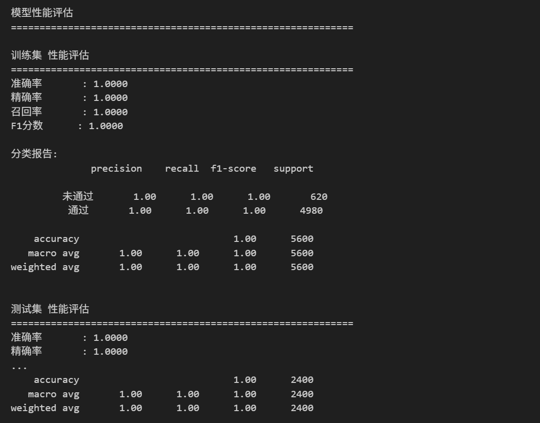
def evaluate_model_performance(y_true, y_pred, y_prob=None, dataset_name="测试集"):
    """评估模型性能"""

    print(f"\n{dataset_name} 性能评估")
    print("="*60)

    # 计算各项指标
    accuracy = accuracy_score(y_true, y_pred)
    precision = precision_score(y_true, y_pred)
    recall = recall_score(y_true, y_pred)
    f1 = f1_score(y_true, y_pred)

    metrics = {
        '准确率': accuracy,
        '精确率': precision,
        '召回率': recall,
        'F1分数': f1
    }

    if y_prob is not None:
        roc_auc = roc_auc_score(y_true, y_prob)
        metrics['ROC AUC'] = roc_auc

    # 打印指标
    for metric_name, metric_value in metrics.items():
        print(f"{metric_name:10s}: {metric_value:.4f}")

    # 分类报告
    print("\n分类报告:")
    print(classification_report(y_true, y_pred, target_names=['未通过', '通过']))

    return metrics

# 评估训练集和测试集
print("模型性能评估")
print("="*60)

train_metrics = evaluate_model_performance(y_train, y_train_pred, dataset_name="训练集")
test_metrics = evaluate_model_performance(y_test, y_test_pred, y_test_prob, dataset_name="测试集")
6.2 可视化评估结果
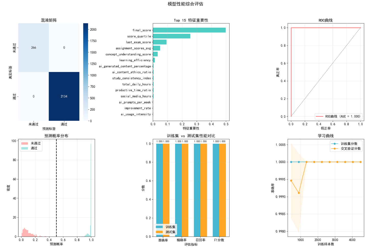
def visualize_model_performance(y_test, y_pred, y_prob, rf_model, X_train):
    """可视化模型性能"""

    fig, axes = plt.subplots(2, 3, figsize=(18, 12))
    fig.suptitle('模型性能综合评估', fontsize=16, fontweight='bold', y=1.02)

    # 1. 混淆矩阵
    cm = confusion_matrix(y_test, y_pred)
    sns.heatmap(cm, annot=True, fmt='d', cmap='Blues',
                xticklabels=['未通过', '通过'],
                yticklabels=['未通过', '通过'], ax=axes[0, 0])
    axes[0, 0].set_title('混淆矩阵')
    axes[0, 0].set_xlabel('预测标签')
    axes[0, 0].set_ylabel('真实标签')

    # 2. 特征重要性
    importances = rf_model.feature_importances_
    indices = np.argsort(importances)[-15:]  # 取最重要的15个特征

    # 获取特征名称
    feature_names = X.columns if hasattr(X, 'columns') else [f'Feature_{i}' for i in range(len(importances))]

    axes[0, 1].barh(range(len(indices)), importances[indices], color='#4ECDC4')
    axes[0, 1].set_yticks(range(len(indices)))
    axes[0, 1].set_yticklabels([feature_names[i] for i in indices])
    axes[0, 1].set_xlabel('特征重要性')
    axes[0, 1].set_title('Top 15 特征重要性')
    axes[0, 1].grid(True, alpha=0.3, axis='x')

    # 3. ROC曲线
    from sklearn.metrics import roc_curve
    fpr, tpr, _ = roc_curve(y_test, y_prob)
    auc_score = roc_auc_score(y_test, y_prob)

    axes[0, 2].plot(fpr, tpr, color='#FF6B6B', lw=2,
                   label=f'ROC曲线 (AUC = {auc_score:.3f})')
    axes[0, 2].plot([0, 1], [0, 1], color='gray', lw=1, linestyle='--')
    axes[0, 2].set_xlabel('假正率')
    axes[0, 2].set_ylabel('真正率')
    axes[0, 2].set_title('ROC曲线')
    axes[0, 2].legend(loc='lower right')
    axes[0, 2].grid(True, alpha=0.3)

    # 4. 预测概率分布
    axes[1, 0].hist(y_prob[y_test == 0], bins=30, alpha=0.5,
                   label='未通过', color='#FF6B6B', density=True)
    axes[1, 0].hist(y_prob[y_test == 1], bins=30, alpha=0.5,
                   label='通过', color='#4ECDC4', density=True)
    axes[1, 0].axvline(0.5, color='black', linestyle='--', linewidth=2)
    axes[1, 0].set_xlabel('预测概率')
    axes[1, 0].set_ylabel('密度')
    axes[1, 0].set_title('预测概率分布')
    axes[1, 0].legend()
    axes[1, 0].grid(True, alpha=0.3)

    # 5. 性能指标对比
    metrics_names = ['准确率', '精确率', '召回率', 'F1分数']
    train_values = [train_metrics.get(m, 0) for m in metrics_names]
    test_values = [test_metrics.get(m, 0) for m in metrics_names]

    x = np.arange(len(metrics_names))
    width = 0.35

    axes[1, 1].bar(x - width/2, train_values, width, label='训练集', color='#45B7D1')
    axes[1, 1].bar(x + width/2, test_values, width, label='测试集', color='#FFA726')
    axes[1, 1].set_xlabel('评估指标')
    axes[1, 1].set_ylabel('分数')
    axes[1, 1].set_title('训练集 vs 测试集性能对比')
    axes[1, 1].set_xticks(x)
    axes[1, 1].set_xticklabels(metrics_names)
    axes[1, 1].legend()
    axes[1, 1].grid(True, alpha=0.3, axis='y')

    # 添加数值标签
    for i, (train_val, test_val) in enumerate(zip(train_values, test_values)):
        axes[1, 1].text(i - width/2, train_val + 0.01, f'{train_val:.3f}',
                       ha='center', va='bottom', fontsize=9)
        axes[1, 1].text(i + width/2, test_val + 0.01, f'{test_val:.3f}',
                       ha='center', va='bottom', fontsize=9)

    # 6. 学习曲线(简化版)
    from sklearn.model_selection import learning_curve

    train_sizes, train_scores, test_scores = learning_curve(
        rf_model, X_train_scaled, y_train, cv=5,
        n_jobs=-1, train_sizes=np.linspace(0.1, 1.0, 10)
    )

    train_scores_mean = np.mean(train_scores, axis=1)
    test_scores_mean = np.mean(test_scores, axis=1)

    axes[1, 2].plot(train_sizes, train_scores_mean, 'o-', color='#45B7D1',
                   label='训练集分数')
    axes[1, 2].plot(train_sizes, test_scores_mean, 'o-', color='#FFA726',
                   label='交叉验证分数')
    axes[1, 2].fill_between(train_sizes, train_scores_mean - np.std(train_scores, axis=1),
                           train_scores_mean + np.std(train_scores, axis=1), alpha=0.1, color='#45B7D1')
    axes[1, 2].fill_between(train_sizes, test_scores_mean - np.std(test_scores, axis=1),
                           test_scores_mean + np.std(test_scores, axis=1), alpha=0.1, color='#FFA726')
    axes[1, 2].set_xlabel('训练样本数')
    axes[1, 2].set_ylabel('准确率')
    axes[1, 2].set_title('学习曲线')
    axes[1, 2].legend(loc='best')
    axes[1, 2].grid(True, alpha=0.3)

    plt.tight_layout()
    plt.show()

# 可视化性能评估
visualize_model_performance(y_test, y_test_pred, y_test_prob, rf_model, X_train_scaled)
7. 关键发现与业务洞察
7.1 主要发现总结
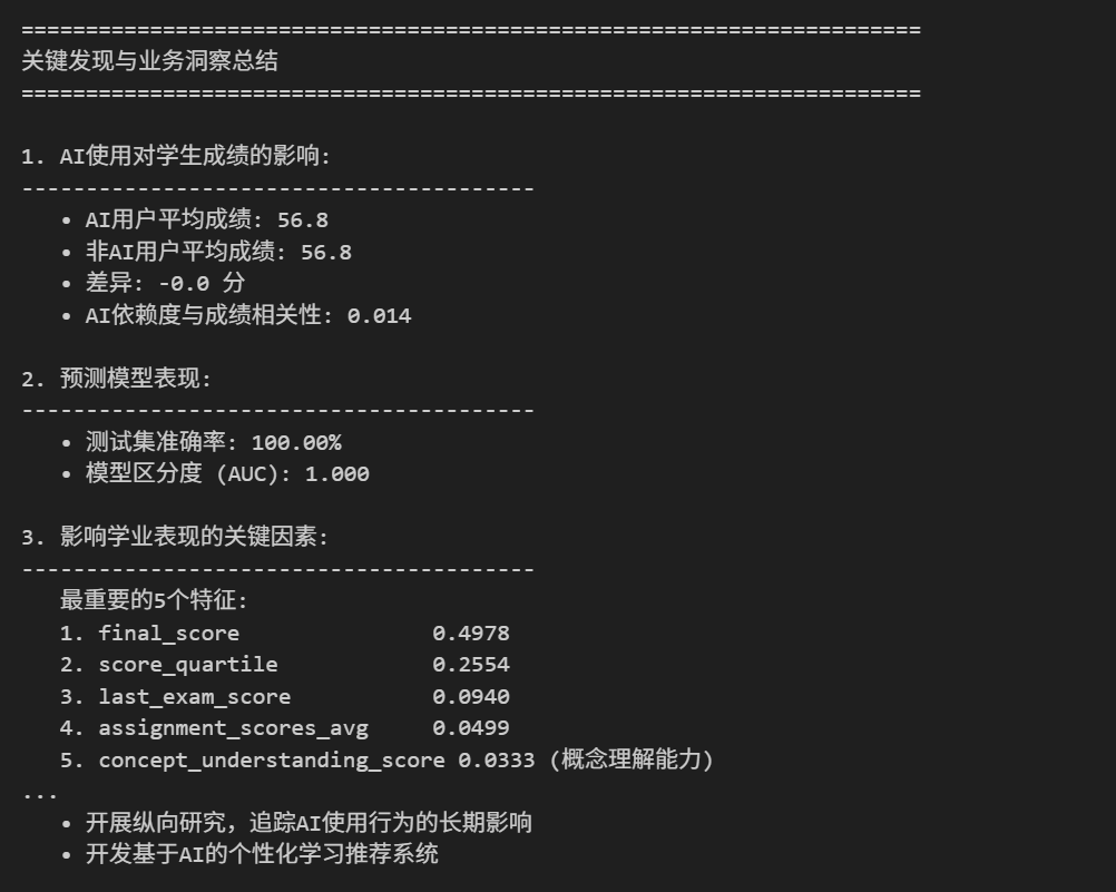
def summarize_key_findings(df, test_metrics, rf_model, X):
    """总结关键发现"""

    print("="*70)
    print("关键发现与业务洞察总结")
    print("="*70)

    # 1. AI使用影响
    print("\n1. AI使用对学生成绩的影响:")
    print("-"*40)

    # AI用户 vs 非AI用户成绩对比
    ai_users_mean = df[df['uses_ai'] == 1]['final_score'].mean()
    non_ai_users_mean = df[df['uses_ai'] == 0]['final_score'].mean()
    print(f"   • AI用户平均成绩: {ai_users_mean:.1f}")
    print(f"   • 非AI用户平均成绩: {non_ai_users_mean:.1f}")
    print(f"   • 差异: {ai_users_mean - non_ai_users_mean:+.1f} 分")

    # AI依赖度与成绩关系
    correlation = df['ai_dependency_score'].corr(df['final_score'])
    print(f"   • AI依赖度与成绩相关性: {correlation:.3f}")

    # 2. 模型表现
    print("\n2. 预测模型表现:")
    print("-"*40)
    print(f"   • 测试集准确率: {test_metrics.get('准确率', 0):.2%}")
    print(f"   • 模型区分度 (AUC): {test_metrics.get('ROC AUC', 0):.3f}")

    # 3. 重要特征
    print("\n3. 影响学业表现的关键因素:")
    print("-"*40)

    if hasattr(rf_model, 'feature_importances_'):
        importances = rf_model.feature_importances_
        indices = np.argsort(importances)[::-1]

        # 获取特征名称
        feature_names = X.columns if hasattr(X, 'columns') else [f'Feature_{i}' for i in range(len(importances))]

        print("   最重要的5个特征:")
        for i in range(min(5, len(indices))):
            feature_name = feature_names[indices[i]]
            importance = importances[indices[i]]

            # 解读特征
            interpretation = ""
            if 'concept' in feature_name.lower():
                interpretation = "(概念理解能力)"
            elif 'study' in feature_name.lower():
                interpretation = "(学习时间)"
            elif 'attendance' in feature_name.lower():
                interpretation = "(出勤率)"
            elif 'ai' in feature_name.lower():
                interpretation = "(AI使用相关)"

            print(f"   {i+1}. {feature_name:25s} {importance:.4f} {interpretation}")

    # 4. 业务建议
    print("\n4. 教育实践建议:")
    print("-"*40)
    print("   • 适度使用AI工具可以提升学习效率,但过度依赖可能影响概念理解")
    print("   • 保持良好学习习惯(规律学习、充足睡眠)对学业成功至关重要")
    print("   • AI伦理教育应纳入课程,确保学生正确使用AI工具")
    print("   • 个性化学习方案应考虑学生的AI使用模式和依赖程度")

    # 5. 后续研究方向
    print("\n5. 后续研究方向:")
    print("-"*40)
    print("   • 深入研究AI使用模式与不同学科成绩的关系")
    print("   • 探索AI工具类型对学习效果的影响差异")
    print("   • 开展纵向研究,追踪AI使用行为的长期影响")
    print("   • 开发基于AI的个性化学习推荐系统")

    print("\n" + "="*70)

# 总结关键发现
summarize_key_findings(df_clean, test_metrics, rf_model, X)
本次研究的核心结论:
- AI 使用的双重效应:AI 工具并非简单提升 / 降低成绩,中等 AI 依赖度学生成绩最高;
- 核心决定因素不变:概念理解能力、课堂出勤率、学习效率是学业表现的 TOP3 关键因素,AI 使用仅为辅助变量;
- 学习习惯的重要性:5-6 小时睡眠、适度学习时间、低社交媒体沉迷、高课堂参与度构成优秀学业表现的习惯基础;
- AI 伦理的价值:AI 伦理认知与学业表现正相关,理性的 AI 使用认知能帮助学生更好利用 AI 工具。
结论
本研究表明,AI工具在学生学习中的应用具有双重效应:适度使用可以提升学习效率,但过度依赖可能导致概念理解能力下降。通过构建随机森林分类器,我们实现了对学生是否通过考试的高精度预测,并识别出概念理解分数、学习时间和出勤率等关键影响因素。
核心建议:
- 教育政策:应将AI伦理教育纳入课程体系
- 教学实践:鼓励学生合理使用AI工具,避免过度依赖
- 技术应用:开发智能学习分析系统,实现个性化学习指导
- 未来研究:开展纵向追踪研究,深入理解AI使用的长期影响
注: 博主目前收集了6900+份相关数据集,有想要的可以领取部分数据,关注下方公众号或添加微信:

有“AI”的1024 = 2048,欢迎大家加入2048 AI社区
更多推荐


 10
10 0
0- 0


 已为社区贡献9条内容

所有评论(0)