手搓大模型体验

Llama2 架构总览

Llama2 遵循了 GPT 系列开创的 Decoder-Only 架构。这意味着它完全由 Transformer 解码器层堆叠而成，天然适用于自回归的文本生成任务。

Llama2 的设计

• 预归一化（Pre-Normalization）：与经典 Transformer 的后归一化不同，输入在进入注意力层和前馈网络之前，都会先经过一次 RMS Norm。这被认为是提升大模型训练稳定性的关键（我们曾提到过，GPT-2/3 正是转向 Pre-Norm 解决了深层网络的训练难题）。
• 组件升级：支持 Grouped-Query Attention（GQA）（如 Llama2-70B 采用 1；小模型可视为 n_kv_heads == n_heads 的 MHA 特例），前馈网络采用 SwiGLU，归一化使用 RMSNorm。
• 旋转位置编码（RoPE）：图中可见，位置信息并非在输入端与词嵌入相加，而是在注意力层内部，通过 RoPE 操作动态地施加于查询（Q）和键（K）向量之上。
• 残差连接：每个子层（注意力层和前馈网络）的输出都通过残差连接（+号）与子层的输入相加，保留了原始信息流。

Llama2数据流

1. 输入嵌入：将 token_ids 转换为词向量。
2. N x Transformer 层堆叠：数据依次通过 N 个相同的 Transformer Block。

• 预归一化：在进入子层之前，先进行一次 RMSNorm。
• 注意力子系统：包含旋转位置编码、分组查询注意力（GQA） 和 KV 缓存机制。
• 前馈网络子系统：采用 SwiGLU 激活函数。

3. 最终归一化与输出：在所有层之后，进行最后一次 RMSNorm，并通过一个线性层将特征映射到词汇表 logits。

关键组件代码实现

预归一化（src/norm.py）

# code/C6/llama2/src/norm.py
class RMSNorm(nn.Module):
    def __init__(self, dim: int, eps: float = 1e-6):
        super().__init__()
        self.eps = eps
        self.weight = nn.Parameter(torch.ones(dim)) # 对应公式中的 gamma

    def _norm(self, x: torch.Tensor) -> torch.Tensor:
        # 核心计算：x * (x^2的均值 + eps)的平方根的倒数
        return x * torch.rsqrt(x.pow(2).mean(dim=-1, keepdim=True) + self.eps)

    def forward(self, x: torch.Tensor) -> torch.Tensor:
        out = self._norm(x.float()).type_as(x)
        return out * self.weight

# 单元测试
if __name__ == "__main__":
    # 准备参数和输入
    batch_size, seq_len, dim = 4, 16, 64
    x = torch.randn(batch_size, seq_len, dim)

    # 初始化并应用 RMSNorm
    norm = RMSNorm(dim)
    output = norm(x)

    # 验证输出形状
    print("--- RMSNorm Test ---")
    print("Input shape:", x.shape)
    print("Output shape:", output.shape)

• _norm 方法精确地实现了 RMSNorm 的核心公式。
• self.eps 是一个为了防止除以零而添加的小常数，保证了数值稳定性。

旋转位置编码代码实现（src/rope.py）

def precompute_freqs_cis(dim: int, end: int, theta: float = 10000.0) -> torch.Tensor:
    # 1. 计算频率：1 / (theta^(2i/dim))
    freqs = 1.0 / (theta ** (torch.arange(0, dim, 2)[: (dim // 2)].float() / dim))
    # 2. 生成位置序列 t = [0, 1, ..., end-1]
    t = torch.arange(end, device=freqs.device)
    # 3. 计算相位：t 和 freqs 的外积
    freqs = torch.outer(t, freqs).float()
    # 4. 转换为复数形式 (cos(theta) + i*sin(theta))
    freqs_cis = torch.polar(torch.ones_like(freqs), freqs)
    return freqs_cis
    
def reshape_for_broadcast(freqs_cis: torch.Tensor, x: torch.Tensor) -> torch.Tensor:
    ndim = x.ndim
    shape = [d if i == 1 or i == ndim - 1 else 1 for i, d in enumerate(x.shape)]
    return freqs_cis.view(*shape)
    
def apply_rotary_emb(
    xq: torch.Tensor,
    xk: torch.Tensor,
    freqs_cis: torch.Tensor,
) -> tuple[torch.Tensor, torch.Tensor]:
    # 将 Q/K 向量视为复数
    xq_ = torch.view_as_complex(xq.float().reshape(*xq.shape[:-1], -1, 2))
    xk_ = torch.view_as_complex(xk.float().reshape(*xk.shape[:-1], -1, 2))
    
    # 准备广播
    freqs_q = reshape_for_broadcast(freqs_cis, xq_)  # 针对 Q 的广播视图
    
    # 复数乘法即为旋转
    xq_out = torch.view_as_real(xq_ * freqs_q).flatten(3)
    
    # K 向量可能与 Q 向量有不同的头数（GQA），所以需单独生成广播视图
    freqs_k = reshape_for_broadcast(freqs_cis, xk_)
    xk_out = torch.view_as_real(xk_ * freqs_k).flatten(3)
    return xq_out.type_as(xq), xk_out.type_as(xq)

# 单元测试
if __name__ == "__main__":
    # 准备参数和输入
    batch_size, seq_len, n_heads, n_kv_heads, head_dim = 4, 16, 8, 2, 16
    dim = n_heads * head_dim
    n_rep = n_heads // n_kv_heads

    # --- Test precompute_freqs_cis ---
    print("--- Test precompute_freqs_cis ---")
    freqs_cis = precompute_freqs_cis(dim=head_dim, end=seq_len * 2)
    print("freqs_cis shape:", freqs_cis.shape)

    # --- Test apply_rotary_emb ---
    print("\n--- Test apply_rotary_emb ---")
    xq = torch.randn(batch_size, seq_len, n_heads, head_dim)
    xk = torch.randn(batch_size, seq_len, n_kv_heads, head_dim)
    freqs_cis_slice = freqs_cis[:seq_len]
    xq_out, xk_out = apply_rotary_emb(xq, xk, freqs_cis_slice)
    print("xq shape (in/out):", xq.shape, xq_out.shape)
    print("xk shape (in/out):", xk.shape, xk_out.shape)

分组查询注意力代码实现(src/attention.py)

# code/C6/llama2/src/rope.py
def repeat_kv(x: torch.Tensor, n_rep: int) -> torch.Tensor:
    batch_size, seq_len, n_kv_heads, head_dim = x.shape
    if n_rep == 1:
        return x
    return (
        x[:, :, :, None, :]
        .expand(batch_size, seq_len, n_kv_heads, n_rep, head_dim)
        .reshape(batch_size, seq_len, n_kv_heads * n_rep, head_dim)
    )
    
class GroupedQueryAttention(nn.Module):
    def __init__(self, dim: int, n_heads: int, n_kv_heads: int | None = None, ...):
        ...
        self.n_local_heads = n_heads
        self.n_local_kv_heads = n_kv_heads
        self.n_rep = self.n_local_heads // self.n_local_kv_heads # Q头与KV头的重复比
        ...
        self.wq = nn.Linear(dim, n_heads * self.head_dim, bias=False)
        self.wk = nn.Linear(dim, n_kv_heads * self.head_dim, bias=False)
        self.wv = nn.Linear(dim, n_kv_heads * self.head_dim, bias=False)
        ...

    def forward(self, x, start_pos, freqs_cis, mask):
        xq = self.wq(x).view(batch_size, seq_len, self.n_local_heads, self.head_dim)
        xk = self.wk(x).view(batch_size, seq_len, self.n_local_kv_heads, self.head_dim)
        xv = self.wv(x).view(batch_size, seq_len, self.n_local_kv_heads, self.head_dim)

        xq, xk = apply_rotary_emb(xq, xk, freqs_cis=freqs_cis)
        
        # ... KV Cache 逻辑 ...

        keys = repeat_kv(keys, self.n_rep)   # <-- 关键步骤
        values = repeat_kv(values, self.n_rep) # <-- 关键步骤

        scores = torch.matmul(xq.transpose(1, 2), keys.transpose(1, 2).transpose(2, 3)) / ...
        
        
# 单元测试
if __name__ == "__main__":
    # 准备参数和输入
    batch_size, seq_len, dim = 4, 16, 128
    n_heads, n_kv_heads = 8, 2
    head_dim = dim // n_heads

    # 初始化注意力模块
    attention = GroupedQueryAttention(
        dim=dim,
        n_heads=n_heads,
        n_kv_heads=n_kv_heads,
        max_batch_size=batch_size,
        max_seq_len=seq_len,
    )

    # 准备输入
    x = torch.randn(batch_size, seq_len, dim)
    freqs_cis = precompute_freqs_cis(dim=head_dim, end=seq_len * 2)
    freqs_cis_slice = freqs_cis[:seq_len]

    # 执行前向传播
    output = attention(x, start_pos=0, freqs_cis=freqs_cis_slice)

    # 验证输出形状
    print("--- GroupedQueryAttention Test ---")
    print("Input shape:", x.shape)
    print("Output shape:", output.shape)

SwiGLU 前馈网络代码实现（src/ffn.py）

class FeedForward(nn.Module):
    def __init__(self, dim: int, hidden_dim: int, multiple_of: int, ...):
        super().__init__()
        # hidden_dim 计算，并用 multiple_of 对齐以提高硬件效率
        hidden_dim = int(2 * hidden_dim / 3)
        ...
        hidden_dim = multiple_of * ((hidden_dim + multiple_of - 1) // multiple_of)

        self.w1 = nn.Linear(dim, hidden_dim, bias=False) # 对应 W
        self.w2 = nn.Linear(hidden_dim, dim, bias=False) # 对应 W2
        self.w3 = nn.Linear(dim, hidden_dim, bias=False) # 对应 V

    def forward(self, x: torch.Tensor) -> torch.Tensor:
        # F.silu(self.w1(x)) 实现了 swish(xW)
        # * self.w3(x) 实现了门控机制
        return self.w2(torch.nn.functional.silu(self.w1(x)) * self.w3(x))
        
# 单元测试
# code/C6/llama2/src/ffn.py
if __name__ == "__main__":
    # 准备参数和输入
    batch_size, seq_len, dim = 4, 16, 128
    
    # 初始化 FFN 模块
    ffn = FeedForward(
        dim=dim,
        hidden_dim=4 * dim,
        multiple_of=256,
        ffn_dim_multiplier=None
    )

    # 准备输入
    x = torch.randn(batch_size, seq_len, dim)

    # 执行前向传播
    output = ffn(x)

    # 验证输出形状
    print("--- FeedForward (SwiGLU) Test ---")
    print("Input shape:", x.shape)
    print("Output shape:", output.shape)

模型组装与前向传播(src/transformer.py)

# TransformerBlock: 这是构成 Llama2 的基本单元
class TransformerBlock(nn.Module):
    def __init__(self, layer_id: int, ...):
        ...
        self.attention = GroupedQueryAttention(...)
        self.feed_forward = FeedForward(...)
        self.attention_norm = RMSNorm(...)
        self.ffn_norm = RMSNorm(...)

    def forward(self, x, start_pos, freqs_cis, mask):
        # 预归一化 + 残差连接
        h = x + self.attention(self.attention_norm(x), start_pos, freqs_cis, mask)
        out = h + self.feed_forward(self.ffn_norm(h))
        return out
        
# LlamaTransformer: 顶层模型，负责堆叠 TransformerBlock 并处理输入输出。
class LlamaTransformer(nn.Module):
    def __init__(self, vocab_size: int, ...):
        ...
        self.tok_embeddings = nn.Embedding(vocab_size, dim)
        self.layers = nn.ModuleList([TransformerBlock(...) for i in range(n_layers)])
        self.norm = RMSNorm(dim, eps=norm_eps)
        self.output = nn.Linear(dim, vocab_size, bias=False)
        self.register_buffer("freqs_cis", precompute_freqs_cis(...))

    def forward(self, tokens: torch.Tensor, start_pos: int) -> torch.Tensor:
        h = self.tok_embeddings(tokens)
        
        # 1. 准备 RoPE 旋转矩阵
        freqs_cis = self.freqs_cis[start_pos : start_pos + seq_len]

        # 2. 准备因果掩码 (Causal Mask)
        mask = None
        if seq_len > 1:
            mask = torch.full((seq_len, seq_len), float("-inf"), device=tokens.device)
            mask = torch.triu(mask, diagonal=1)
            # 考虑 KV Cache 的偏移
            mask = torch.hstack([torch.zeros((seq_len, start_pos), ...), mask]).type_as(h)

        # 3. 循环通过所有 TransformerBlock
        for layer in self.layers:
            h = layer(h, start_pos, freqs_cis, mask)
        
        h = self.norm(h)
        logits = self.output(h).float()
        return logits

整体验证

import torch
from src.transformer import LlamaTransformer

def main() -> None:
    # 使用小尺寸参数，便于 CPU/GPU 都能快速跑通
    model = LlamaTransformer(
        vocab_size=1000,
        dim=256,
        n_layers=2,
        n_heads=8,
        n_kv_heads=2,
        multiple_of=64,
        ffn_dim_multiplier=None,
        norm_eps=1e-6,
        max_batch_size=4,
        max_seq_len=64,
    )

    # 构造随机 token 序列并执行前向
    batch_size, seq_len = 2, 16
    tokens = torch.randint(0, 1000, (batch_size, seq_len))
    logits = model(tokens, start_pos=0)

    # 期望: [batch_size, seq_len, vocab_size]
    print("logits shape:", tuple(logits.shape))

if __name__ == "__main__":
    main()

MoE架构

稠密模型（Dense Model）:lama2、GPT-3
混合专家模型（Mixture of Experts, MoE）:MoE 技术通过一种 “稀疏激活” 的机制，兼具了大规模参数的知识容量与极低的推理成本。Mistral 8x7B 等模型的出现，更是证明了 MoE 在开源大模型领域的巨大潜力，使其成为当前最受关注的技术方向之一

来源

最早的 MoE 思想可以追溯到 1991 年 Michael Jordan 和 Geoffrey Hinton 发表的经典论文《Adaptive Mixture of Local Experts》

大模型时代的 MoE

入 Transformer 时代后，MoE 技术成为了突破模型规模瓶颈的关键。Google 在这一领域进行了密集的探索，通过 GShard、Switch Transformer 和 GLaM 等一系列工作，确立了现代大规模 MoE 的技术范式。

MoE 架构的创新与实践

随着开源社区的活跃，MoE 技术不再是科技巨头的专属。Mistral 8x7B 和 DeepSeek-R1 的出现，分别在中等规模和超大规模上证明了开源 MoE 模型的强大实力，标志着 MoE 技术进入了全面普及和深度创新的新阶段。

Mistral 8x7B的架构总览

Mistral 8x7B (Mixtral) 7 在开源大语言模型中成功实践了 MoE 架构，有力地证明了合理设计的稀疏模型即使不需要万亿参数，也能超越同量级的稠密模型。

• 架构参数：它拥有约 470 亿（47B） 的总参数量（Sparse Parameters），但对于每个 Token，仅激活 130 亿（13B） 参数（Active Parameters）。这使得它在推理时拥有 13B 模型的计算速度，却能发挥出 47B 模型的知识容量。需要注意的是，虽然计算量较小，但由于所有专家参数都需要加载到内存中，其显存占用（VRAM Usage）依然是 47B 模型级别的。
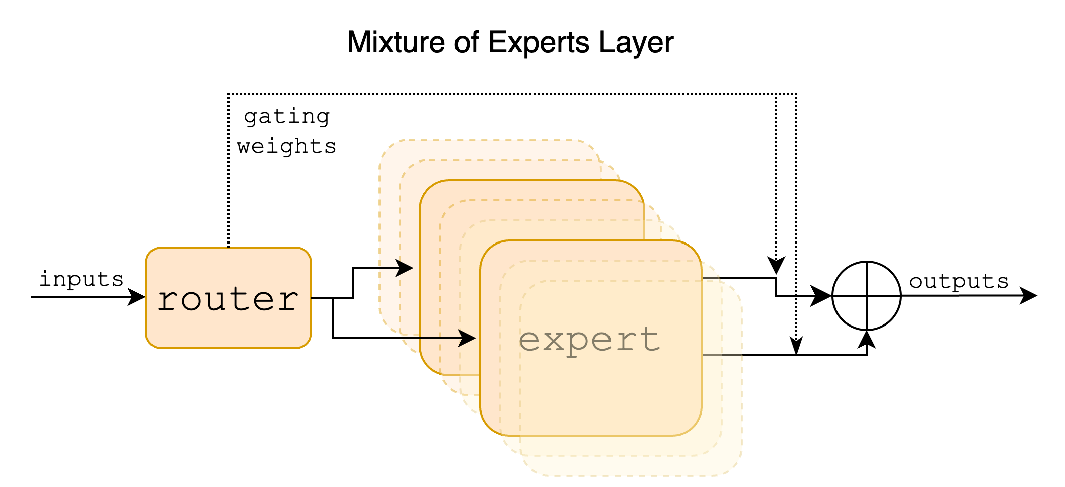
• 路由机制：每一层包含 8 个专家（Experts），采用标准的 Top-2 Routing 策略。如图 6-10 所示，每个输入 Token 会被 Router 网络分配给 8 个专家中的 2 个，这两个专家的输出经过加权求和后作为该层的最终输出。这种机制巧妙地在增加模型容量（更多专家）的同时，保持了极低的推理成本（只激活 2 个）。
  
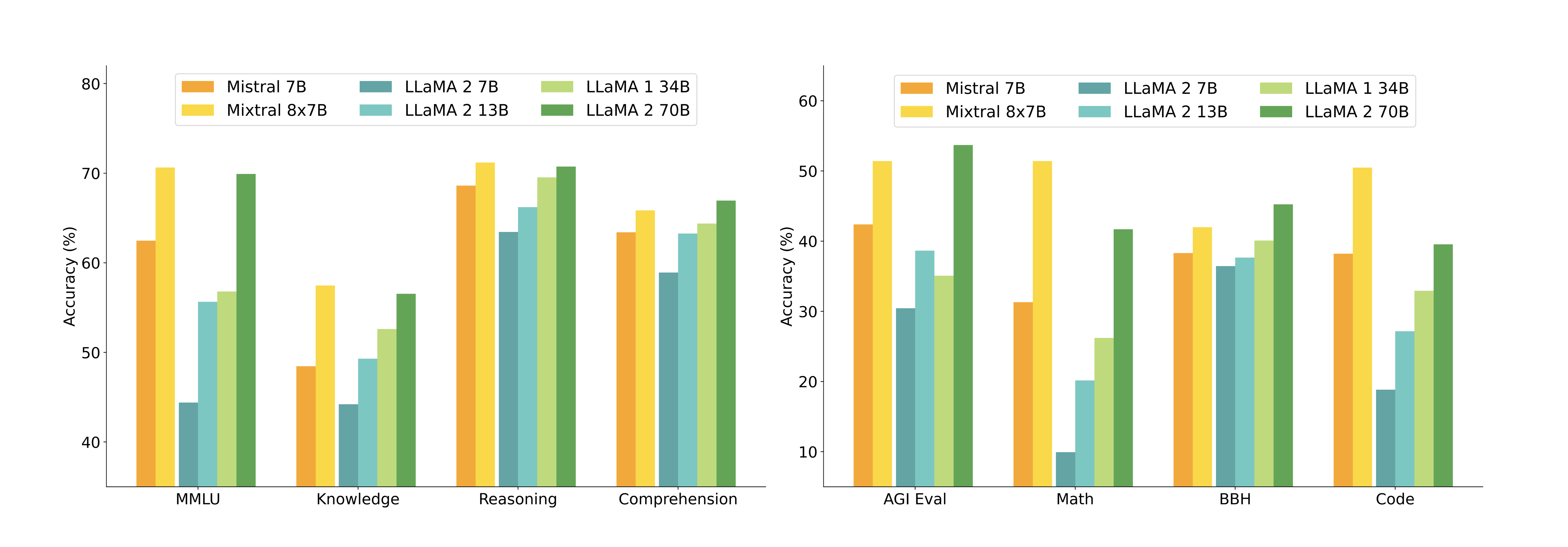
• 性能表现：在 GSM8K（数学）、MMLU（综合知识）、HumanEval（代码）等基准测试上，Mistral 8x7B 以 13B 的活跃参数量超越了稠密的 Llama 2 70B 以及 GPT-3.5。如图 6-11，Mistral 8x7B（黄色柱状图）在几乎所有任务上都包围或持平了 Llama 2 70B（绿色柱状图），特别是在数学和代码生成任务上，其优势尤为显著。
• 长上下文能力：Mistral 8x7B 支持 32k 的上下文长度，并且在长文本信息检索（Passkey Retrieval）任务中表现出了 100% 的召回率，证明了 MoE 架构在处理长序列时依然稳健。
  

DeepSeekMoE 与 DeepSeek-R1

如果说 Mistral 开启了开源 MoE 模型的大门，那么 DeepSeek-R1 8（及其基座 DeepSeek-V3 9）则将开源 MoE 模型的性能推向了与当时顶尖闭源模型（如 OpenAI o1）比肩的高度。DeepSeek 在 MoE 架构上进行了更深度的创新，提出了 DeepSeekMoE 10 架构，目标是解决传统 Top-k 路由中的“知识冗余”和“专业化不足”问题。

代码实战

实现 MoE 层

class MoE(nn.Module):
    def __init__(self, dim: int, hidden_dim: int, multiple_of: int, ffn_dim_multiplier: Optional[float], num_experts: int = 8, top_k: int = 2):
        super().__init__()
        self.num_experts = num_experts
        self.top_k = top_k
        # 门控网络：决定每个 Token 去往哪个专家
        self.gate = nn.Linear(dim, num_experts, bias=False)
        # 专家列表：创建 num_experts 个独立的 FeedForward 网络
        self.experts = nn.ModuleList([
            FeedForward(dim, hidden_dim, multiple_of, ffn_dim_multiplier)
            for _ in range(num_experts)
        ])

    def forward(self, x: torch.Tensor) -> torch.Tensor:
        # x: (batch_size, seq_len, dim)
        B, T, D = x.shape
        x_flat = x.view(-1, D)
        
        # 1. 门控网络
        gate_logits = self.gate(x_flat) # (B*T, num_experts)
        # 2. Top-k 路由
        weights, indices = torch.topk(gate_logits, self.top_k, dim=-1)
        weights = F.softmax(weights, dim=-1) # 归一化权重
        
        output = torch.zeros_like(x_flat)
        
        for i, expert in enumerate(self.experts):
            # 3. 找出所有选中当前专家 i 的 token 索引
            batch_idx, k_idx = torch.where(indices == i)
            
            if len(batch_idx) == 0:
                continue
                
            # 4. 取出对应的输入进行计算
            expert_input = x_flat[batch_idx]
            expert_out = expert(expert_input)
            
            # 5. 获取对应的权重
            expert_weights = weights[batch_idx, k_idx].unsqueeze(-1) # (num_selected, 1)
            
            # 6. 将结果加权累加回输出张量
            output.index_add_(0, batch_idx, expert_out * expert_weights)
            
        return output.view(B, T, D)

替换 TransformerBlock

from .ffn import FeedForward, MoE # 导入 MoE

class TransformerBlock(nn.Module):
    def __init__(
        # ... args ...
    ):
        super().__init__()
        # ...
        
        # 修改：使用 MoE 替换标准的 FeedForward
        self.feed_forward = MoE(
            dim=dim,
            hidden_dim=4 * dim,
            multiple_of=multiple_of,
            ffn_dim_multiplier=ffn_dim_multiplier,
            num_experts=8,  # 定义8个专家
            top_k=2,        # 每个Token激活2个专家
        )

参考代码仓

https://github.com/datawhalechina/base-llm