BEVWORLD: A MULTIMODAL WORLD SIMULATOR FOR AUTONOMOUS DRIVING VIA SCENE-LEVEL BEV LATENTS

Yumeng Zhang Shi Gong Kaixin Xiong Xiaoqing Ye† Xiaofan Li Xiao Tan Fan Wang Jizhou Huang† * Hua Wu Haifeng Wang Baidu Inc., China {zhangyumeng04,gongshi,yexiaoqing,huangjizhou01}@baidu.com

ABSTRACT

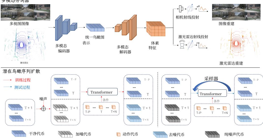
World models have attracted increasing attention in autonomous driving for their ability to forecast potential future scenarios. In this paper, we propose BEVWorld, a novel framework that transforms multimodal sensor inputs into a unified and compact Bird’s Eye View (BEV) latent space for holistic environment modeling. The proposed world model consists of two main components: a multi-modal tokenizer and a latent BEV sequence diffusion model. The multi-modal tokenizer first encodes heterogeneous sensory data, and its decoder reconstructs the latent BEV tokens into LiDAR and surround-view image observations via ray-casting rendering in a self-supervised manner. This enables joint modeling and bidirectional encoding-decoding of panoramic imagery and point cloud data within a shared spatial representation. On top of this, the latent BEV sequence diffusion model performs temporally consistent forecasting of future scenes, conditioned on high-level action tokens, enabling scene-level reasoning over time. Extensive experiments demonstrate the effectiveness of BEVWorld on autonomous driving benchmarks, showcasing its capability in realistic future scene generation and its benefits for downstream tasks such as perception and motion prediction. Code will be released soon.

1 INTRODUCTION

Driving World Models (DWMs) have become an increasingly critical component in autonomous driving, enabling vehicles to forecast future scenes based on current or historical observations. Beyond augmenting training data, DWMs offer realistic simulated environments that support end-to-end reinforcement learning. These models empower self-driving systems to simulate diverse scenarios and make high-quality decisions.

Recent advancements in general image and video generation have significantly accelerated the development of generative models for autonomous driving. Most studies in this field typically leverage open-source models pretrained on large-scale 2D image or video datasets Rombach et al. (2022); Blattmann et al. (2023), adapting their strong generative capabilities to the driving domain. These works Wang et al. (2023a); Li et al. (2024); Gao et al. (2023) either extend the temporal dimensions of image generation models or directly fine-tune video foundation models, achieving impressive 2D generation results with only limited driving data.

However, realistic simulation of driving scenarios requires 3D spatial modeling, which cannot be sufficiently captured by 2D representations alone. Some DWMs adopt 3D representations as intermediate states Zheng et al. (2024) or predict 3D structures directly, such as point clouds Zhang et al. (2024). Nevertheless, these approaches often focus on a single 3D modality and struggle to accommodate the multi-sensor, multi-modal nature of modern autonomous driving systems. Due to the inherent heterogeneity in multi-modal data, integrating 2D images or videos with 3D structures into a unified generative model remains an open challenge.

BEVWORLD：一种通过场景级 BEV 潜变量的多模态自动驾驶世界模拟器

Yumeng Zhang Shi Gong Kaixin Xiong Xiaoqing Ye† Xiaofan Li Xiao Tan FanWang JizhouHuang† ${}^{\ast }$ Hua Wu Haifeng WangBaiduInc., 中 国{zhangyumeng04,gongshi,yexiaoqing,huangjizhou01}@baidu.com

摘要

世界模型因其预测潜在未来场景的能力在自动驾驶领域受到越来越多关注。在本文中，我们提出了BEVWorld，一个将多模态传感器输入转化为统一且紧凑的鸟瞰图（BEV）潜在空间以实现整体环境建模的新框架。所提出的世界模型由两部分主要组件组成：一个多模态分词器和一个潜在 BEV 序列扩散模型。多模态分词器首先对异构感知数据进行编码，其解码器通过自监督的射线投射渲染将潜在 BEV 令牌重构为激光雷达和环视图像观测。这使得在共享的空间表示内可以对全景影像和点云数据进行联合建模及双向编码—解码。在此基础上，潜在 BEV 序列扩散模型在高层动作令牌的条件下执行时间一致的未来场景预测，从而实现基于场景的时序推理。大量实验表明 BEVWorld 在自动驾驶基准测试中的有效性，展示了其在真实感未来场景生成方面的能力及其对感知和运动预测等下游任务的益处。代码将很快开源。

1 引言

驾驶世界模型（Driving World Models，DWMs）已成为自动驾驶中日益关键的组成部分，能够基于当前或历史观测预测未来场景。除了增强训练数据外，DWMs 还提供了支持端到端强化学习的逼真模拟环境。这些模型使自动驾驶系统能够模拟多样化场景并做出高质量的决策。

近年来，通用图像与视频生成的进展显著加速了自动驾驶生成模型的发展。本领域的大多数研究通常利用在大规模二维图像或视频数据集上预训练的开源模型 Rombach et al. (2022);Blattmann 等（2023），将其强大的生成能力适配到驾驶领域。这些工作 Wang et al.(2023a); Li et al. (2024); Gao et al. (2023) 要么扩展图像生成模型的时序维度，要么直接微调视频基础模型，在仅有有限驾驶数据的情况下也取得了令人印象深刻的二维生成结果。

然而，对驾驶场景的真实模拟需要三维空间建模，仅靠二维表示无法充分捕捉。部分DWM 将三维表示作为中间状态（Zheng et al. (2024)），或直接预测三维结构，例如点云（Zhang 等（2024））。尽管如此，这些方法常常只关注单一三维模态，难以兼顾现代自动驾驶系统的多传感器、多模态特性。由于多模态数据固有的异构性，将二维图像或视频与三维结构整合到统一的生成模型中仍然是一个开放的挑战。

Moreover, many existing models adopt end-to-end architectures to model the transition from past to future Yang et al. (2024b); Zhou et al. (2025). However, high-quality generation of both images and point clouds depends on the joint modeling of low-level pixel or voxel details and high-level behavioral dynamics of scene elements such as vehicles and pedestrians. Naively forecasting future states without explicitly decoupling these two levels often limits model performance.

To address these challenges, we propose BEVWorld—a multi-modal world model that transforms heterogeneous sensor data into a unified bird’s-eye-view (BEV) representation, enabling actionconditioned future prediction within a shared spatial space. BEVWorld consists of two decoupled components: a multi-modal tokenizer network and a latent BEV sequence diffusion model. The tokenizer focuses on low-level information compression and high-fidelity reconstruction, while the diffusion model predicts high-level behavior in a temporally structured manner.

The core of our multi-modal tokenizer lies in projecting raw sensor inputs into a unified latent BEV space. This is achieved by transforming visual features into 3D space and aligning them with LiDAR-based geometry via a self-supervised autoencoder. To reconstruct the original multi-modal data, we lift the BEV latents back to 3D voxel representations and apply ray-based rendering Yang et al. (2023) to synthesize high-resolution images and point clouds.

The latent BEV diffusion model focuses on forecasting future BEV frames. Thanks to the abstraction provided by the tokenizer, this task is greatly simplified. Specifically, we employ a diffusion-based generative approach combined with a spatiotemporal transformer, which denoises the latent BEV sequence into precise future predictions conditioned on planned actions.

Our key contributions are as follows:

• We propose a novel multi-modal tokenizer that unifies visual semantics and 3D geometry into a BEV representation. By leveraging a rendering-based reconstruction method, we ensure high BEV quality and validate its effectiveness through ablations, visualizations, and downstream tasks. • We design a latent diffusion-based world model that enables synchronized generation of multi-view images and point clouds. Extensive experiments on the nuScenes and Carla datasets demonstrate our model’s superior performance in multi-modal future prediction.

2 RELATED WORKS

2.1 WORLD MODEL

This part mainly reviews the application of world models in the autonomous driving area, focusing on scenario generation as well as the planning and control mechanism. If categorized by the key applications, we divide the sprung-up world model works into two categories. (1) Driving Scene Generation. The data collection and annotation for autonomous driving are high-cost and sometimes risky. In contrast, world models find another way to enrich unlimited, varied driving data due to their intrinsic self-supervised learning paradigms. GAIA-1 Hu et al. (2023) adopts multi-modality inputs collected in the real world to generate diverse driving scenarios based on different prompts (e.g., changing weather, scenes, traffic participants, vehicle actions) in an autoregressive prediction manner, which shows its ability of world understanding. ADriver-I Jia et al. (2023) combines the multimodal large language model and a video latent diffusion model to predict future scenes and control signals, which significantly improves the interpretability of decision-making, indicating the feasibility of the world model as a fundamental model. MUVO Bogdoll et al. (2023) integrates LiDAR point clouds beyond videos to predict future driving scenes in the representation of images, point clouds, and 3D occupancy. Further, Copilot4D Zhang et al. (2024) leverages a discrete diffusion model that operates on BEV tokens to perform 3D point cloud forecasting and OccWorld Zheng et al. (2023) adopts a GPT-like generative architecture for 3D semantic occupancy forecast and motion planning. DriveWorld Min et al. (2024) and UniWorld Min et al. (2023) approach the world model as 4D scene understanding task for pre-training for downstream tasks. (2) Planning and Control. MILE Hu et al. (2022) is the pioneering work that adopts a model-based imitation learning approach for joint dynamics future environment and driving policy learning in autonomous driving. DriveDreamer Wang et al. (2023a) offers a comprehensive framework to utilize 3D structural information such as HDMap and 3D box to predict future driving videos and driving actions. Beyond the single front 此外，许多现有模型采用端到端架构来建模从过去到未来的演变（Yang et al. (2024b)； Zhou et al. (2025)）。然而，高质量地生成图像和点云依赖于对低级像素或体素细节与高 级场景元素行为动态（如车辆和行人）之间的联合建模。未经明确解耦这两个层面而简单 地预测未来状态，往往会限制模型性能。

为了解决这些挑战，我们提出了BEVWorld——一种多模态世界模型，它将异构传感器数据转化为统一的鸟瞰图（BEV）表示，从而在共享的空间中实现基于动作的未来预测。BEVWorld 由两个解耦的组件组成：多模态分词器网络和潜在 BEV 序列扩散模型。分词器侧重于低层信息的压缩与高保真重建，而扩散模型则以时序化的方式预测高级行为。

我们多模态分词器的核心在于将原始传感器输入投影到统一的潜在 BEV 空间。这通过将视觉特征变换到三维空间并通过自监督自编码器与基于激光雷达的几何信息对齐来实现。为了重建原始多模态数据，我们将 BEV 潜变量抬升回三维体素表示，并采用基于光线的渲染（Yang et al. (2023)）来合成高分辨率图像和点云。

潜在 BEV 扩散模型专注于预测未来的 BEV 帧。得益于分词器提供的抽象，这一任务被大大简化。具体而言，我们采用基于扩散的生成方法结合时空 Transformer，通过对潜在BEV 序列去噪，在给定规划动作的条件下生成精确的未来预测。

我们的主要贡献如下：

• 我们提出了一种新颖的多模态分词器，将视觉语义和三维几何统一为 BEV 表示。通过利用基于渲染的重建方法，确保了高质量的 BEV，并通过消融实验、可视化和下游任务验证了其有效性。• 我们设计了一种基于潜空间扩散的世界模型，能够同步生成多视图图像和点云。在 nuScenes 和Carla 数据集上的大量实验表明，我们的模型在多模态未来预测任务上具有优越的性能。

2 相关工作

2.1 世界模型

这部分主要回顾世界模型在自动驾驶领域的应用，聚焦于场景生成以及规划与控制机制。若按关键应用分类，我们将新涌现的世界模型工作划分为两类。 (1) 驾驶场景生成。自动驾驶的数据采集和标注成本高昂且有时存在风险。相比之下，世界模型凭借其固有的自监督学习范式，为丰富无限、多样的驾驶数据提供了另一种途径。GAIA‑1 Hu et al. (2023) 采用在真实世界中收集的多模态输入，基于不同提示（例如改变天气、场景、交通参与者、车辆动作）以自回归预测的方式生成多样的驾驶场景，展示了其对世界的理解能力。ADriver‑I Jia et al. (2023) 将多模态大语言模型与视频潜在扩散模型结合，用于预测未来场景和控制信号，显著提高了决策的可解释性，表明将世界模型作为基础模型的可行性。MUVO Bogdoll et al. (2023) 在视频之外整合了激光雷达点云，以图像、点云和三维占据的表示形式预测未来驾驶场景。进一步地，Copilot4D Zhang et al. (2024) 利用在 BEV 令牌上运行的离散扩散模型来执行三维点云预测，而 OccWorld Zheng et al. (2023) 采用类 GPT 生成架构进行三维语义占据预测和运动规划。DriveWorld Min et al. (2024) 和 UniWorld Min et al. (2023) 将世界模型视为用于下游任务预训练的 4D 场景理解任务。 (2) 规划与控制。MILE Hu et al. (2022) 是开创性工作，采用基于模型的模仿学习方法在自动驾驶中联合学习未来环境动力学和驾驶策略。DriveDreamerWang et al. (2023a) 提供了一个综合框架，利用诸如 HDMap 和 3D 盒子等三维结构信息来预测未来驾驶视频和驾驶动作。超越单一前

view generation, DriveDreamer-2 Zhao et al. (2024) further produces multi-view driving videos based on user descriptions. TrafficBots Zhang et al. (2023) develops a world model for multimodal motion prediction and end-to-end driving, by facilitating action prediction from a BEV perspective. Drive-WM Wang et al. (2023b) generates controllable multiview videos and applies the world model to safe driving planning to determine the optimal trajectory according to the image-based rewards.

2.2 VIDEO DIFFUSION MODEL

World model can be regarded as a sequence-data generation task, which belongs to the realm of video prediction. Many early methods Hu et al. (2022; 2023) adopt VAE Kingma & Welling (2013) and auto-regression Chen et al. (2024) to generate future predictions. However, the VAE suffers from unsatisfactory generation quality, and the auto-regressive method has the problem of cumulative error. Thus, many researchers switch to study on diffusion-based future prediction methods Zhao et al. (2024); Li et al. (2023), which achieves success in the realm of video generation recently and has ability to predict multiple future frames simultaneously. This part mainly reviews the related methods of video diffusion model.

The standard video diffusion model Ho et al. (2022) takes temporal noise as input, and adopts the UNet Ronneberger et al. (2015) with temporal attention to obtain denoised videos. However, this method requires high training costs and the generation quality needs further improvement. Subsequent methods are mainly improved along these two directions. In view of the high training cost problem, LVDMHe et al. (2022) and Open-Sora Lab & etc. (2024) methods compress the video into a latent space through schemes such as VAE or VideoGPT Yan et al. (2021), which reduces the video capacity in terms of spatial and temporal dimensions. In order to improve the generation quality of videos, stable video diffusion Blattmann et al. (2023) proposes a multi-stage training strategy, which adopts image and low-resolution video pretraining to accelerate the model convergence and improve generation quality. GenAD Yang et al. (2024a) introduces the causal mask module into UNet to predict plausible futures following the temporal causality. VDT Lu et al. (2023a) and Sora Brooks et al. (2024) replace the traditional UNet with a spatial-temporal transformer structure. The powerful scale-up capability of the transformer enables the model to fit the data better and generates more reasonable videos. Vista Gao et al. (2024), built upon GenAD, integrates a large amount of additional data and introduces structural and motion losses to enhance dynamic modeling and structural fidelity, thereby enabling high-resolution, high-quality long-term scene generation. Subsequent works further extend the prediction horizon Guo et al. (2024); Hu et al. (2024); Li et al. (2025) and unify prediction with perception Liang et al. (2025).

3 METHOD

In this section, we delineate the model structure of BEVWorld. The overall architecture is illustrated in Figure 1. Given a sequence of multi-view image and Lidar observations {ot−P,⋅⋅⋅,ot−1,ot,ot+1,⋅⋅⋅,ot+N}\left\{ o _ { t - P } , \cdot \cdot \cdot , o _ { t - 1 } , o _ { t } , o _ { t + 1 } , \cdot \cdot \cdot , o _ { t + N } \right\}{ot−P​,⋅⋅⋅,ot−1​,ot​,ot+1​,⋅⋅⋅,ot+N​} where $o_t$ is the current observation, $+/-$ represent the future/past observations and $P/N$ is the number of past/future observations, we aim to predict {ot+1,⋅⋅⋅,ot+N}\left\{ o _ { t + 1 } , \cdot \cdot \cdot , o _ { t + N } \right\}{ot+1​,⋅⋅⋅,ot+N​} with the condition {ot−P,⋅⋅⋅,ot−1,ot}\left\{ o _ { t - P } , \cdot \cdot \cdot , o _ { t - 1 } , o _ { t } \right\}{ot−P​,⋅⋅⋅,ot−1​,ot​} . In view of the high computing costs of learning a world model in original observation space, a multi-modal tokenizer is proposed to compress the multi-view image and Lidar information into a unified BEV space by frame. The encoder-decoder structure and the self-supervised reconstruction loss promise proper geometric and semantic information is well stored in the BEV representation. This design exactly provides a sufficiently concise representation for the world model and other downstream tasks. Our world model is designed as a diffusion-based network to avoid the problem of error accumulating as those in an autoregressive fashion. It takes the ego motion and {xt−P,⋅⋅⋅,xt−1,xt}\{ x _ { t - P } , \cdot \cdot \cdot , x _ { t - 1 } , x _ { t } \}{xt−P​,⋅⋅⋅,xt−1​,xt​} , i.e. the BEV representation of $\{\overline{o_{t-P}},\cdot \cdot \cdot ,o_{t-1},o_t\}$ , as condition to learn the noise {ϵt+1,⋅⋅⋅,ϵt+N}\left\{ \epsilon _ { t + 1 } , \cdot \cdot \cdot , \epsilon _ { t + N } \right\}{ϵt+1​,⋅⋅⋅,ϵt+N​} added to {xt+1,⋅⋅⋅,xt+N}\{ x _ { t + 1 } , \cdot \cdot \cdot , x _ { t + N } \}{xt+1​,⋅⋅⋅,xt+N​} in the training process. In the testing process, a DDIM Song et al. (2020) scheduler is applied to restore the future BEV token from pure noises. Next we use the decoder of multi-modal tokenizer to render future multi-view images and Lidar frames out.

视图生成，DriveDreamer‑2 Zhao et al. (2024) 进一步根据用户描述生成多视角驾驶视频。TrafficBots Zhang et al. (2023) 为多模态运动预测和端到端驾驶构建了世界模型，通过aBEV 视角促进动作预测。Drive‑WM Wang et al. (2023b) 生成功能可控的多视角视频，并将世界模型应用于安全驾驶规划，以根据基于图像的奖励确定最优轨迹。

2.2 视频扩散模型

世界模型可被视为序列数据生成任务，属于视频预测范畴。许多早期方法 Hu 等（2022；2023）采用变分自编码器 VAE Kingma & Welling（2013）和自回归 Chen 等（2024）来生成未来预测。然而，VAE 在生成质量上表现不佳，自回归方法则存在累计误差问题。因此，许多研究者转而研究基于扩散的未来预测方法 Zhao 等（2024）；Li 等（2023），该类方法近年来在视频生成领域取得了成功，并具备同时预测多帧未来帧的能力。本节主要回顾视频扩散模型的相关方法。

标准视频扩散模型 Ho 等（2022）以时序噪声为输入，采用带有时间注意力的 UNetRonneberger 等（2015）来获得去噪后的视频。然而，该方法训练成本高且生成质量仍需提升。后续方法主要沿这两个方向改进。针对高训练成本问题，LVDM He 等（2022）和Open‑Sora Lab 等（2024）的方法通过 VAE 或 VideoGPT Yan 等（2021）等方案将视频压缩到潜在空间，从而在空间和时间维度上减少视频容量。为提升视频生成质量，stable video diffusion Blattmann 等（2023）提出了多阶段训练策略，采用图像和低分辨率视频预训练以加速模型收敛并提高生成质量。GenAD Yang 等（2024a）将因果掩码模块引入 UNet，以遵循时间因果性预测合理的未来。VDT Lu et al. (2023a) 和 SoraBrooks 等（2024）用时空 Transformer 结构替代传统 UNet。Transformer 强大的扩展能力使模型更好地拟合数据并生成更合理的视频。基于 GenAD 的 Vista Gao 等（2024）整合了大量额外数据并引入结构与运动损失以增强动态建模和结构保真度，从而实现高分辨率、高质量的长期场景生成。后续工作进一步扩展了预测视野 Guo 等（2024）；Hu 等（2024）；Li 等（2025），并将预测与感知统一 Liang 等（2025）。

3 方法

在本节中，我们阐述了 BEVWorld 的模型结构。整体架构如图1 所示。给定一系列多视角图像和激光雷达观测 {ot−P,⋅⋅⋅,ot−1,ot,ot+1,⋅⋅⋅,ot+N}\left\{ o _ { t - P } , \cdot \cdot \cdot , o _ { t - 1 } , o _ { t } , o _ { t + 1 } , \cdot \cdot \cdot , o _ { t + N } \right\}{ot−P​,⋅⋅⋅,ot−1​,ot​,ot+1​,⋅⋅⋅,ot+N​} ，其中 $o_t$ 是当前观测， $+/-$ 表示未来/过去的观测， $P/N$ 是过去/未来观测的数量，我们的目标是预测 {ot+1,⋅⋅⋅,ot+N}\left\{ o _ { t + 1 } , \cdot \cdot \cdot , o _ { t + N } \right\}{ot+1​,⋅⋅⋅,ot+N​} ，条件为 {ot−P,⋅⋅⋅,ot−1,ot}c\{ o _ { t - P } , \cdot \cdot \cdot , o _ { t - 1 } , o _ { t } \} _ { c }{ot−P​,⋅⋅⋅,ot−1​,ot​}c​ 。鉴于在原始观测空间中学习世界模型的计算代价很高，我们提出了一个多模态分词器，将多视角图像和激光雷达信息按帧压缩到统一的 BEV 空间。编码器‑解码器结构和自监督重建损失保证了几何和语义信息能够被良好地保存在 BEV 表示中。该设计恰好为世界模型和其他下游任务提供了一个足够简洁的表示。我们的世界模型被设计为一个基于扩散的网络，以避免像自回归方式那样的误差累积问题。它以自车运动和 {xt−P,⋅⋅⋅,xt−1,xt}\{ x _ { t - P } , \cdot \cdot \cdot , x _ { t - 1 } , x _ { t } \}{xt−P​,⋅⋅⋅,xt−1​,xt​} ，即 {ot−P,⋅⋅⋅,ot−1,ot}\left\{ o _ { t - P } , \cdot \cdot \cdot , o _ { t - 1 } , o _ { t } \right\}{ot−P​,⋅⋅⋅,ot−1​,ot​} 的 BEV 表征，作为条件，在训练过程中学习添加到 {xt+1,⋅⋅⋅,xt+N}\{ x _ { t + 1 } , \cdot \cdot \cdot , x _ { t + N } \}{xt+1​,⋅⋅⋅,xt+N​} 上的噪声 {ϵt+1,⋅⋅⋅,ϵt+N}\{ \epsilon _ { t + 1 } , \cdot \cdot \cdot , \epsilon _ { t + N } \}{ϵt+1​,⋅⋅⋅,ϵt+N​} 。在测试过程中，应用了 DDIMSong et al. (2020) 调度器从纯噪声中还原未来的 BEV 代币。随后我们使用多模态分词器的解码器渲染出未来的多视角图像和激光雷达帧。

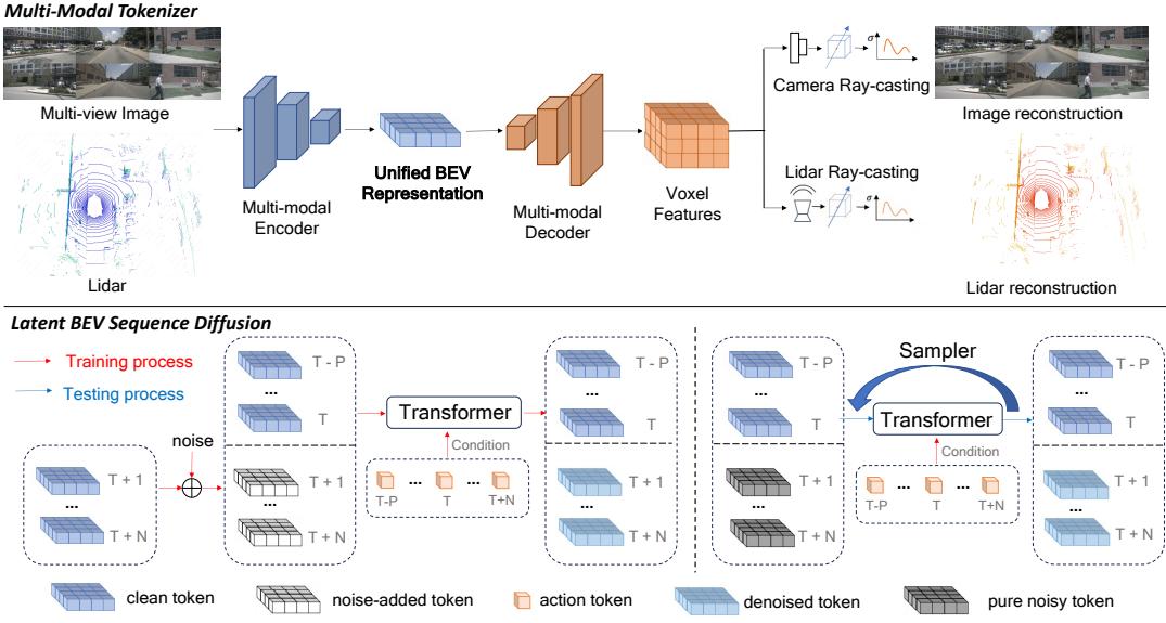
Figure 1: An overview of our method BEVWorld. BEVWorld consists of the multi-modal tokenizer and the latent BEV sequence diffusion model. The tokenizer first encodes the image and Lidar observations into BEV tokens, then decodes the unified BEV tokens to reconstructed observations by NeRF rendering strategies. Latent BEV sequence diffusion model predicts future BEV tokens with corresponding action conditions by a Spatial-Temporal Transformer. The multi-frame future BEV tokens are obtained by a single inference, avoiding the cumulative errors of auto-regressive methods.

3.1 MULTI-MODAL TOKENIZER

Our designed multi-modal tokenizer contains three parts: a BEV encoder network, a BEV Decoder network and a multi-modal rendering network. The structure of BEV encoder network is illustrated in the Figure 2. To make the multi-modal network as homogeneous as possible, we adopt the Swin-Transformer Liu et al. (2021) network as the image backbone to extract multi-image features. For Lidar feature extraction, we first split point cloud into pillars Lang et al. (2019) on the BEV space. Then we use the Swin-Transformer network as the Lidar backbone to extract Lidar BEV features. We fuse the Lidar BEV features and the multi-view images features with a deformable-based transformer Zhu et al. (2020). Specifically, we sample $K(K=4)$ points in the height dimension of pillars and project these points onto the image to sample corresponding image features. The sampled image features are treated as values and the Lidar BEV features is served as queries in the deformable attention calculation. Considering the future prediction task requires low-dimension inputs, we further compress the fused BEV feature into a low-dimensional $C^{\prime }=4$ ) BEV feature.

For BEV decoder, there is an ambiguity problem when directly using a decoder to restore the images and Lidar since the fused BEV feature lacks height information. To address this problem, we first convert BEV tokens into 3D voxel features through stacked layers of upsampling and swin-blocks. And then we use voxelized NeRF-based ray rendering to restore the multi-view images and Lidar point cloud.

The multi-modal rendering network can be elegantly segmented into two distinct components, image reconstruction network and Lidar reconstruction network. For image reconstruction network, we first get the ray $\mathbf{r}(t)=\mathbf{o}+t\mathbf{d}$ , which shooting from the camera center o to the pixel center in direction $\mathbf{d}$ Then we uniformly sample a set of points $\{(x_i,y_i,z_i){\}}_{i=1}^{N_r}$ along the ray, where $N_r(N_r=150)$ is the total number of points sampled along a ray. Given a sampled point $(x_i,y_i,z_i)$ , the corresponding features ${\mathbf{v}}_i$ are obtained from the voxel feature according to its position. Then, all the sampled features in a ray are aggregated as pixel-wise feature descriptor (Eq. 1).

$$\mathbf{v}(\mathbf{r})=\sum _{i=1}^{N_r}{w}_i{\mathbf{v}}_{\mathbf{i}},w_i={\alpha }_i\prod _{j=1}^{i-1}(1-{\alpha }_j),{\alpha }_i=\sigma (\mathrm{MLP}({\mathbf{v}}_{\mathbf{i}}))$$

多模态分词器

图1：我们的方法 BEVWorld 概览。BEVWorld 由多模态分词器和潜在 BEV 序列扩散模型组成。分词器首先将图像和激光雷达观测编码为 BEV 令牌，然后通过 NeRF 渲染策略将统一的BEV 令牌解码为重建的观测。潜在 BEV 序列扩散模型通过时空变换器在对应的动作条件下预测未来的 BEV 令牌。多帧未来 BEV 令牌可通过单次推理获得，避免了自回归方法的累积误差。

3.1 多模态分词器

我们设计的多模态分词器包含三部分：BEV 编码器网络、BEV 解码器网络和多模态渲染网络。BEV 编码器网络的结构如图2 所示。为了使多模态网络尽可能同质化，我们采用Swin‑Transformer Liu et al. (2021) 网络作为图像主干网络来提取多图像特征。对于激光雷达特征提取，我们首先在 BEV 空间将点云划分为 pillars Lang et al. (2019)。然后我们使用Swin‑Transformer 网络作为激光雷达主干网络以提取激光雷达 BEV 特征。我们用基于可变形注意力的 Transformer Zhu et al. (2020) 融合激光雷达 BEV 特征和多视角图像特征。具体地，我们在 pillars 的高度维度采样 $K(K=4)$ 个点，并将这些点投影到图像上以采样相应的图像特征。采样到的图像特征作为值，而激光雷达 BEV 特征作为可变形注意力计算中的查询。考虑到未来预测任务需要低维输入，我们进一步将融合的 BEV 特征压缩为低维的l $C^{\prime }=4,$ )BEV 特征。

对于 BEV 解码器，直接使用解码器恢复图像和激光雷达会存在歧义问题，因为融合后的BEV 特征缺乏高度信息。为了解决此问题，我们首先通过堆叠的上采样层和 Swin 块将BEV 令牌转换为三维体素特征。然后使用基于体素的 NeRF 光线渲染来恢复多视图图像和雷达点云。

多模态渲染网络可以优雅地分成两个独立的组成部分：图像重建网络和激光雷达重建网络。对于图像重建网络，我们首先得到光线 $\mathbf{r}(t)=\mathbf{o}+t\mathbf{d}$ ，该光线从相机中心 $\nabla \cdot \mathbf{o}$ 射向像素中心，方向为d。然后我们在光线上均匀采样一组点 $\{(x_i,y_i,z_i){\}}_{i=1}^{N_r}$ ，其中 $N_r(N_r=150)$ 是沿光线采样的点的总数。给定一个采样点 $( x _ { i } , y _ { i } , z _ { i } ) $ ，相应的特征 ${\mathbf{v}}_i$ 根据其位置从体素特征中获得。随后，将一条光线上所有采样到的特征聚合为逐像素特征描述子（公式 1）。

$$\mathbf{v}(\mathbf{r})=\sum _{i=1}^{N_r}{w}_i{\mathbf{v}}_{\mathbf{i}},w_i={\alpha }_i\prod _{j=1}^{i-1}(1-{\alpha }_j),{\alpha }_i=\sigma (\mathrm{MLP}({\mathbf{v}}_{\mathbf{i}}))$$

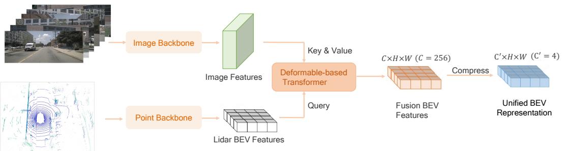
Figure 2: The detailed structure of BEV encoder. The encoder takes as input the multi-view multimodality sensor data. Multimodal information is fused using deformable attention, BEV features are channel-compressed to be compatible with the diffusion models.

We traverse all pixels and obtain the 2D feature map $\mathbf{V}\in {\mathbb{R}}^{H_f\times W_f\times C_f}$ of the image. The 2D feature is converted into the RGB image ${\mathbf{I}}_{\mathbf{g}}\in {\mathbb{R}}^{H\times W\times 3}$ through a CNN decoder. Three common losses are added for improving the quality of generated images, perceptual loss Johnson et al. (2016), GAN loss Goodfellow et al. (2020) and L1 loss. Our full objective of image reconstruction is:

$${\mathcal{L}}_{\mathrm{rgb}}=\Vert {\mathbf{I}}_{\mathbf{g}}-{\mathbf{I}}_{\mathbf{t}}{\Vert }_1+{\lambda }_{\mathrm{perc}}\Vert \sum _{j=1}^{N_{\varphi }}{\varphi }^j({\mathbf{I}}_{\mathbf{g}})-{\varphi }^j({\mathbf{I}}_{\mathbf{t}})\Vert +{\lambda }_{\mathrm{gan}}{\mathcal{L}}_{\mathrm{gan}}({\mathbf{I}}_{\mathbf{g}},{\mathbf{I}}_{\mathbf{t}})$$

where ${\mathbf{I}}_{\mathbf{t}}$ is the ground truth of ${\mathbf{I}}_{\mathbf{g}}$ , ${\varphi }^j$ represents the jth layer of pretrained VGG Simonyan & Zisserman (2014) model, and the definition of ${\mathcal{L}}_{\mathrm{gan}}({\mathbf{I}}_{\mathbf{g}},{\mathbf{I}}_{\mathbf{t}})$ can be found in Goodfellow et al. (2020).

For Lidar reconstruction network, the ray is defined in the spherical coordinate system with inclination $\theta$ and azimuth $\varphi$ . $\theta$ and $\varphi$ are obtained by shooting from the Lidar center to current frame of Lidar point. We sample the points and get the corresponding features in the same way of image reconstruction. Since Lidar encodes the depth information, the expected depth $D_g(\mathbf{r})$ of the sampled points are calculated for Lidar simulation. The depth simulation process and loss function are shown in Eq. 3.

$$D_g(\mathbf{r})=\sum _{i=1}^{N_r}{w}_i{t}_i,{\mathcal{L}}_{\mathrm{Lidar}}=\Vert D_g(\mathbf{r})-D_t(\mathbf{r}){\Vert }_1,$$

where $t_i$ denotes the depth of sampled point from the Lidar center and $D_t(\mathbf{r})$ is the depth ground truth calculated by the Lidar observation.

The Cartesian coordinate of point cloud could be calculated by:

$$(x,y,z)=(D_g(\mathbf{r})\sin \theta \cos \varphi ,D_g(\mathbf{r})\sin \theta \sin \varphi ,D_g(\mathbf{r})\cos \theta )$$

Overall, the multi-modal tokenizer is trained end-to-end with the total loss in Eq. 5:

$${\mathcal{L}}_{\mathrm{Total}}={\mathcal{L}}_{\mathrm{Lidar}}+{\mathcal{L}}_{\mathrm{rgb}}$$

3.2 LATENT BEV SEQUENCE DIFFUSION

Most existing world models Zhang et al. (2024); Hu et al. (2023) adopt autoregression strategy to get longer future predictions, but this method is easily affected by cumulative errors. Instead, we propose latent sequence diffusion framework, which inputs multiple frames of noise BEV tokens and obtains all future BEV tokens simultaneously.

The structure of latent sequence diffusion is illustrated in Figure 1. In the training process, the low-dimensional BEV tokens $\left(x_{t-P},\cdot \cdot \cdot ,x_{t-1},x_t,x_{t+1},\cdot \cdot \cdot ,x_{t+N}\right)$ are firstly obtained from the sensor data. Only BEV encoder in the multi-modal tokenizer is involved in this process and the parameters of multi-modal tokenizer is frozen. To facilitate the learning of BEV token features by the world model module, we standardize the input BEV features along the channel dimension $\left({\overline{x}}_{t-P},\cdot \cdot \cdot ,{\overline{x}}_{t-1},{\overline{x}}_t,{\overline{x}}_{t+1},\cdot \cdot \cdot ,{\overline{x}}_{t+N}\right)$ . Latest history BEV token and current frame BEV token 我们遍历所有像素并得到图像的二维特征图 $\mathbf{V}\in {\mathbb{R}}^{H_f\times W_f\times C_f}$ 。二维特征通过 CNN 解码器被转换为 RGB 图像 ${\mathbf{I}}_{\mathbf{g}}\in {\mathbb{R}}^{H\times W\times 3}$ 。为提高生成图像的质量，加入了三种常用损失：感知损失 Johnson et al. (2016)、生成对抗网络损失 Goodfellow et al. (2020) 和 L1 损失。我们的图像重建完整目标为：

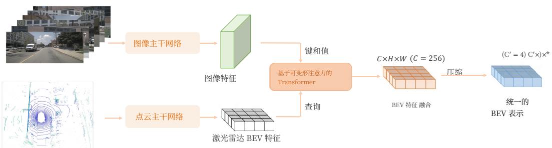
图 2：BEV 编码器的详细结构。编码器将多视角多模态传感器数据作为输入。多模态信息通过可变形注意力进行融合，BEV 特征被通道压缩以与扩散模型兼容。

$${\mathcal{L}}_{\mathrm{rgb}}=\Vert {\mathbf{I}}_{\mathbf{g}}-{\mathbf{I}}_{\mathbf{t}}{\Vert }_1+{\lambda }_{\mathrm{perc}}\Vert \sum _{j=1}^{N_{\varphi }}{\varphi }^j({\mathbf{I}}_{\mathbf{g}})-{\varphi }^j({\mathbf{I}}_{\mathbf{t}})\Vert +{\lambda }_{\mathrm{gan}}{\mathcal{L}}_{\mathrm{gan}}({\mathbf{I}}_{\mathbf{g}},{\mathbf{I}}_{\mathbf{t}})$$

其中 ${\mathbf{I}}_{\mathbf{t}}$ 是 Ig 的真实标签， ${\varphi }^j$ 表示预训练 VGG Simonyan & Zisserman (2014) 模型的第 j层， ${\mathcal{L}}_{\mathrm{gan}}({\mathbf{I}}_{\mathbf{g}},{\mathbf{I}}_{\mathbf{t}})$ 的定义可在 Goodfellow et al. (2020) 中找到。

对于激光雷达重建网络，光线在球面坐标系中定义，具有倾角 $\theta$ 和方位角 ${\varphi }_{\circ }$ 。 $\theta$ 和 $\varphi$ 通过从雷达中心射向当前帧的雷达点获得。我们对这些点进行采样，并以与图像重建相同的方式获取相应的特征。由于雷达编码了深度信息，采样点的期望深度 $D_g(\mathbf{r})$ 会为雷达模拟而计算。深度模拟过程和损失函数在式 3 中给出。

$$D_g(\mathbf{r})=\sum _{i=1}^{N_r}{w}_i{t}_i,{\mathcal{L}}_{\mathrm{Lidar}}=\Vert D_g(\mathbf{r})-D_t(\mathbf{r}){\Vert }_1,$$

其中 $t_i$ 表示从雷达中心采样点的深度， $D_t(\mathbf{r})$ 是由雷达观测计算得到的深度真实值。

点云的笛卡尔坐标可以通过以下公式计算：

$$(x,y,z)=(D_g(\mathbf{r})\sin \theta \cos \varphi ,D_g(\mathbf{r})\sin \theta \sin \varphi ,D_g(\mathbf{r})\cos \theta )$$

总体上，多模态分词器通过式 (5) 中的总损失进行端到端训练：

$${\mathcal{L}}_{\mathrm{Total}}={\mathcal{L}}_{\mathrm{Lidar}}+{\mathcal{L}}_{\mathrm{rgb}}$$

3.2 LATENT BEV SEQUENCEDIFFUSION

大多数现有的世界模型 Zhang 等（2024）；Hu 等（2023）采用自回归策略以获得更长的未来预测，但该方法容易受到累积误差的影响。相反，我们提出了潜在序列扩散框架，该框架输入多帧噪声 BEV 令牌，并同时获得所有未来的 BEV 令牌。

潜在序列扩散的结构如图1所示。在训练过程中，低维的 BEV 令牌(xt−P , · · · , xt−1, xt, xt+1, · · · , xt+N) 首先从传感器数据中获得。此过程中仅多模态分词器中的BEV 编码器参与，多模态分词器的参数被固定。为了便于世界模型模块学习 BEV 令牌特征，我们沿着通道维度对输入 BEV 特征进行标准化 $(x_{t-P},\cdot \cdot \cdot ,x_{t-1},x_t,x_{t+1},\cdot \cdot \cdot ,x_{t+N}{)}_{\circ }$ 。最新的历史 BEV 令牌和当前帧 BEV 令牌

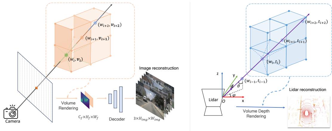
Figure 3: Left: Details of the multi-view images rendering. Trilinear interpolation is applied to the series of sampled points along the ray to obtain weight $w_i$ and feature ${\mathbf{v}}_i$ . {vi}\{ \mathbf { v } _ { i } \}{vi​} are weighted by {wi}\{ w _ { i } \}{wi​} and summed, respectively, to get the rendered image features, which are concatenated and fed into the decoder for $8\times$ upsampling, resulting in multi-view RGB images. Right: Details of Lidar rendering. Trilinear interpolation is also applied to obtain weight $w_i$ and depth $t_i$ . {ti}\{ t _ { i } \}{ti​} are weighted by {wi}\{ w _ { i } \}{wi​} and summed, respectively, to get the final depth of point. Then the point in spherical coordinate system is transformed to the Cartesian coordinate system to get vanilla Lidar point coordinate.

$({\overline{x}}_{t-P},\cdot \cdot \cdot ,{\overline{x}}_{t-1},{\overline{x}}_t)$ d as condit with noise while , wher $({\overline{x}}_{t+1},\cdot \cdot \cdot ,{\overline{x}}_{t+N})$ are diffused to noisyp of diffusion process. $({\overline{x}}_{t+1}^{ϵ},\cdot \cdot \cdot ,{\overline{x}}_{t+N}^{ϵ})$ {ϵt^i}i=t+1t+N\{ \epsilon _ { \hat { t } } ^ { i } \} _ { i = t + 1 } ^ { t + N }{ϵt^i​}i=t+1t+N​ $\hat{t}$

The denoising process is carried out with a spatial-temporal transformer containing a sequence of transformer blocks, the architecture of which is shown in the Figure 4. The input of spatial$\left({\overline{x}}_{t-P},\cdot \cdot \cdot ,{\overline{x}}_{t-1},{\overline{x}}_t,{\overline{x}}_{t+1}^{ϵ},\cdot \cdot \cdot ,{\overline{x}}_{t+N}^{ϵ}\right)$ nation of condition BEV tokens and noisy B. These tokens are modulated with action tokens {ai}i=T−PT+N\{ a _ { i } \} _ { i = T - P } ^ { T + N }{ai​}i=T−PT+N​ More specifically, the input tokens are first passed to temporal attention block for enhancing temporal smoothness. To avoid time confusion problem, we added the causal mask into temporal attention. Then, the output of temporal attention block are sent to spatial attention block for accurate details. The design of spatial attention block foAction token and diffusion timestamp {t^id}i=T−PT+N\{ \hat { t } _ { i } ^ { d } \} _ { i = T - P } ^ { T + N }{t^id​}i=T−PT+N​ ard transformer block criterion Luare concatenated as the condition {ci}i=T−PT+N\{ c _ { i } \} _ { i = T - P } ^ { T + N }{ci​}i=T−PT+N​ a).of diffusion models and then sent to AdaLN Peebles & Xie (2023) (6) to modulate the token features.

$$\mathbf{c}=\mathrm{concat}(\mathbf{a},\hat{\mathbf{t}});\gamma ,\beta =\mathrm{Linear}(\mathbf{c});\mathrm{AdaLN}(\hat{\mathbf{x}},\gamma ,\beta )=\mathrm{LayerNorm}(\hat{\mathbf{x}})\cdot (1+\gamma )+\beta$$

where $\hat{\mathbf{x}}$ is the input features of one transformer block, $\gamma ,\beta$ is the scale and shift of $\mathbf{c}$ .

The output of the Spatial-Temporal transformer is the noise prediction {ϵt^i(x)}i=1N\{ \epsilon _ { \hat { t } } ^ { i } ( \mathbf { x } ) \} _ { i = 1 } ^ { N }{ϵt^i​(x)}i=1N​ , and the loss is shown in Eq. 7.

$${\mathcal{L}}_{\mathrm{diff}}=\Vert {ϵ}_{\hat{\mathbf{t}}}(\mathbf{x})-{ϵ}_{\hat{\mathbf{t}}}{\Vert }_1.$$

In the testing process, normalized history frame and current frame BEV tokens $({\overline{x}}_{t-P},\cdot \cdot \cdot ,{\overline{x}}_{t-1},{\overline{x}}_t)$ and pure noisy tokens $({ϵ}_{t+1},{ϵ}_{t+2},\cdot \cdot \cdot ,{ϵ}_{t+N})$ are concatenated as input to world model. The ego motion token {ai}i=T−PT+N\{ a _ { i } \} _ { i = T - P } ^ { T + N }{ai​}i=T−PT+N​ , spanning from moment $T-P$ to $T+N$ , serve as the conditional inputs. We employ the DDIM Song et al. (2020) schedule to forecast the subsequent BEV tokens. Subsequently, the denormalized operation is applied to the predicted BEV tokens, which are then fed into the BEV decoder and rendering network yielding a comprehensive set of predicted multi-sensor data.

4 EXPERIMENTS

4.1 DATASET

NuScenes Caesar et al. (2020) NuScenes is a widely used autonomous driving dataset, whichcomprises multi-modal data such as multi-view images from 6 cameras and Lidar scans. It includes a$({\overline{x}}_{t-P},\cdot \cdot \cdot ,\overline{x_{t-1}},\overline{x_t})$ 作为条件令牌，而 $(x_{t+1},\cdot \cdot \cdot ,x_{t+N})$ 被扩散为带噪 BEV 令牌$(x_{t+1}^{ϵ},\cdot \cdot \cdot ,x_{t+N}^{ϵ})$ ，噪声为 {ϵt^i}i=t+1t+N\{ \epsilon _ { \hat { t } } ^ { i } \} _ { i = t + 1 } ^ { t + N }{ϵt^i​}i=t+1t+N​ ，其中 ${\hat{\rho }}_t$ 是扩散过程的时间戳。去噪过程由一个时空Transformer 执行，该 Transformer 包含一系列 Transformer 块，其结构见图4。时空Transformer 的输入是条件 BEV 令牌与带噪 BEV 令牌的拼接$({\underline{x}}_{t-P},\cdot \cdot \cdot ,x_{t-1},x_t,x_{t+1}^{ϵ},\cdot \cdot \cdot ,x_{t+N}^{ϵ}{)}_0$ 这些令牌由表示车辆运动和转向的动作令牌 {ai}i=T−PT+N\{ a _ { i } \} _ { i = T - P } ^ { T + N }{ai​}i=T−PT+N​ 进行调制，共同构成时空 Transformer 的输入。更具体地，输入令牌首先被送入时间注意力块以增强时序平滑性。为避免时间混淆问题，我们在时间注意力中加入了因果掩码。随后，时间注意力块的输出被送入空间注意力块以获得精确细节。空间注意力块的设计遵循标准Transformer 块的准则 Lu et al. (2023a)。动作代币与扩散时间戳 {t^id}i=T−PT+N\{ \hat { t } _ { i } ^ { d } \} _ { i = T - P } ^ { T + N }{t^id​}i=T−PT+N​ 被串联作为扩散模型的条件 {ci}i=T−PT+N\{ c _ { i } \} _ { i = T - P } ^ { T + N }{ci​}i=T−PT+N​ ，然后送入 AdaLN Peebles & Xie (2023) (6) 以调节令牌特征。

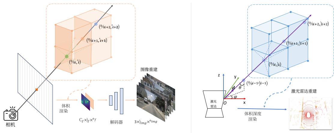
Figure 3: Left：多视角图像渲染的细节。对沿光线采样的一系列点应用三线性插值以获得权重 $w_i$ 和特征 ${\mathbf{v}}_{i\circ }$ 。 {vi}\{ \mathbf { v } _ { i } \}{vi​} 分别按 {wi}\{ w _ { i } \}{wi​} 加权并求和，以得到渲染的图像特征，这些特征被串联并输入解码器进行 $8\times$ 上采样，生成多视角 RGB 图像。Right：激光雷达渲染的细节。同样应用三线性插值以获得权重 $w_i$ 和深度 $t_{i\circ }$ 。 {ti}\{ t _ { i } \}{ti​} 分别按 {wi}\{ w _ { i } \}{wi​} 加权并求和，以得到点的最终深度。然后将点从球面坐标系转换到笛卡尔坐标系以获得基础激光雷达点坐标。

$\mathbf{c}=\mathrm{concat}(\mathbf{a},\hat{\mathbf{t}});\gamma ,\beta =\mathrm{Linear}(\mathbf{c});\mathrm{AdaLN}(\hat{\mathbf{x}},\gamma ,\beta )=\mathrm{LayerNorm}(\hat{\mathbf{x}})\cdot (1+\gamma )+\beta$ 其中 ${\hat{\mu }}_{\mathbf{x}}$ 是一个 Transformer 模块的输入特征， $\gamma ,\beta$ 是 $\mathbf{c}$ 的尺度和平移。时空变换器的输出是噪声预测 {ϵt^i(x)}i=1N\{ \epsilon _ { \hat { t } } ^ { i } ( \mathbf { x } ) \} _ { i = 1 } ^ { N }{ϵt^i​(x)}i=1N​ ，损失如式 7 所示。

$${\mathcal{L}}_{\mathrm{diff}}=\Vert {ϵ}_{\hat{\mathbf{t}}}(\mathbf{x})-{ϵ}_{\hat{\mathbf{t}}}{\Vert }_1.$$

在测试过程中，归一化的历史帧和当前帧 BEV 令牌 $(x_{t-P},\cdot \cdot \cdot ,x_{t-1},x_t)$ 与纯噪声令牌$({ϵ}_{t+1},{ϵ}_{t+2},\cdot \cdot \cdot ,{ϵ}_{t+N})$ 串联作为世界模型的输入。自车运动令牌 {ai}i=T−PT+N\left\{ a _ { i } \right\} _ { i = T - P } ^ { T + N }{ai​}i=T−PT+N​ ，跨越自moment $T-P$ to $T+N$ ，作为条件输入。我们采用 DDIM Song 等（2020）调度方案来预测后续的 BEV 令牌。随后对预测的 BEV 令牌进行反归一化操作，然后将其输入到 BEV 解码器和渲染网络，生成完整的预测多传感器数据。

4 实验

4.1 数据集

NuScenes Caesar et al. (2020) NuScenes 是一个被广泛使用的自动驾驶数据集，包含多模态数据，例如来自6个相机的多视角图像和激光雷达扫描。它包括一个

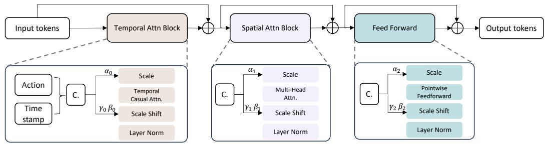
Figure 4: The architecture of Spatial-Temporal transformer block.

total of 700 training videos and 150 validation videos. Each video includes 20 seconds at a frame rate of $12\mathrm{Hz}$ .

Carla Dosovitskiy et al. (2017) The training data is collected in the open-source CARLA simulator at $2\mathrm{Hz}$ , including 8 towns and 14 kinds of weather. We collect 3M frames with four cameras $1600\times$ 900) and one Lidar (32p) for training, and evaluate on the Carla Town05 benchmark, which is the same setting of Shao et al. (2022).

4.2 MULTI-MODAL TOKENIZER

In this section, we explore the impact of different design decisions in the proposed multi-modal tokenizer and demonstrate its effectiveness in the downstream tasks. For multi-modal reconstruction visualization results, please refer to Figure7 and Figure8.

4.2.1 ABLATION STUDIES

Various input modalities and output modalities. The proposed multi-modal tokenizer supports various choice of input and output modalities. We test the influence of different modalities, and the results are shown in Table 1, where L indicates Lidar modality, C indicates multi-view cameras modality, and L&C indicates multi-modal modalities. The combination of Lidar and cameras achieves the best reconstruction performance, which demonstrates that using multi modalities can generate better BEV features. We find that the PSNR metric is somewhat distorted when comparing ground truth images and predicted images. This is caused by the mean characteristics of PSNR metric, which does not evaluate sharpening and blurring well. As shown in Figure 12, though the PSNR of multi modalities is slightly lower than single camera modality method, the visualization of multi modalities is better than single camera modality as the FID metric indicates.

Table 1: Ablations of different modalities.

Input	Output	FID↓	PSNR↑	Chamfer↓
C	C	19.18	26.95	=
C	L	-	1	2.67
L	L	-	-	0.19
L&C	L&C	5.54	25.68	0.15

Table 2: Ablations of rendering methods.

Method	FID↓	PSNR↑	Chamfer↓
(a)	67.28	9.45	0.24
(b)	5.54	25.68	0.15

Rendering approaches. To convert from BEV features into multiple sensor data, the main challenge lies in the varying positions and orientations of different sensors, as well as the differences in imaging (points and pixels). We compared two types of rendering methods: a) attention-based method, which implicitly encodes the geometric projection in the model parameters via global attention mechanism; b) ray-based sampling method, which explicitly utilizes the sensor’s pose information and imaging geometry. The results of the methods (a) and (b) are presented in Table 2. Method (a) faces with a significant performance drop in multi-view reconstruction, indicating that our ray-based sampling approach reduces the difficulty of view transformation, making it easier to achieve training convergence. Thus we adopt ray-based sampling method for generating multiple sensor data.

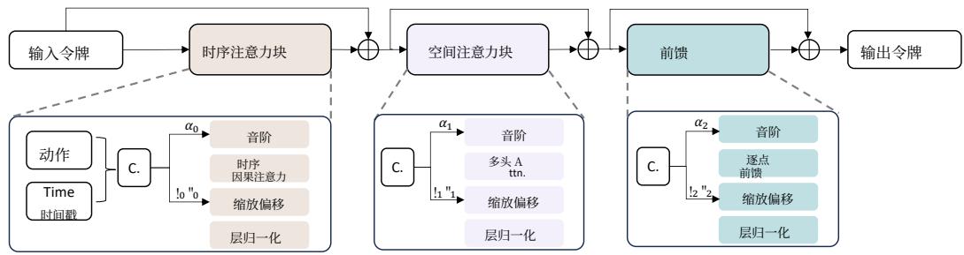
图4：时空变换器模块的架构。

共计700个训练视频和150个验证视频。每个视频包含20秒，帧率为 $12{\mathrm{Hz}}_{\circ }$

Carla Dosovitskiy et al. (2017) 训练数据在开源 CARLA 模拟器中以 $2\mathrm{Hz}$ 频率采集，包含 8 个城镇和 14 种天气。我们为训练收集了 3M 帧，使用四台相机（ $1600\times 900$ ）和一台激光雷达（32p），并在 Carla Town05 基准上进行评估，这与 Shao et al. (2022) 的设置相同。

4.2 多模态分词器

在本节中，我们探索所提出的多模态分词器中不同设计决策的影响，并展示其在下游任务中的有效性。有关多模态重建的可视化结果，请参见图7 和图8。

4.2.1 消融研究

各种输入模态和输出模态。所提出的多模态分词器支持多种输入和输出模态的选择。我们测试了不同模态的影响，结果如表 1 所示，其中 L 表示激光雷达模态，C 表示多视角相机模态，L&C 表示激光雷达与相机模态。激光雷达与相机的组合实现了最佳的重建性能，这表明使用多模态可以生成更好的 BEV 特征。我们发现，在比较真实图像和预测图像时，PSNR 指标在某种程度上存在失真。这是由 PSNR 指标的均值特性引起的，该指标不能很好地评估锐化和模糊。如图12 所示，尽管多模态的 PSNR 略低于单相机模态的方法，但如FID 指标所示，多模态的可视化效果优于单相机模态。

表 1：不同模态的消融。

输入	输出	FID↓	PSNR↑	Chamfer↓
C	C	19.18	26.95	-
C	L	-	-	2.67
L	L	=		0.19
L与C	L与C	5.54	25.68	0.15

表 2：渲染 方法 的消融实验。

方法	FID↓	PSNR↑	Chamfer↓
(a)	67.28	9.45	0.24
(b)	5.54	25.68	0.15

Renderingapproaches.要将 BEV 特征转换为多传感器数据，主要挑战在于不同传感器位置和朝向的差异，以及成像（点和像素）方面的差异。我们比较了两类渲染方法：a) 基于注意力的方法，通过全局注意力机制在模型参数中隐式编码几何投影；b) 基于光线的采样方法，显式利用传感器的位姿信息和成像几何。方法 (a) 和 (b) 的结果见表 2。方法 (a) 在多视角重建上出现显著的性能下降，表明我们的基于光线的采样方法降低了视图变换的难度，更易于实现训练收敛。因此我们采用基于光线的采样方法来生成多传感器数据。

4.2.2 BENEFIT FOR DOWNSTREAM TASKS

3D Detection. To verify our proposed method is effective for downstream tasks when used in the pre-train stage, we conduct experiments on the nuScenes 3D detection benchmark. For the model structure, in order to maximize the reuse of the structure of our multi-modal tokenizer, the encoder in the downstream 3D detection task is kept the same with the encoder of the tokenizer described in 3. We use a BEV encoder attached to the tokenizer encoder for further extracting BEV features. We design a UNet-style network with the Swin-transformer Liu et al. (2021) layers as the BEV encoder. As for the detection head, we adopt query-based head Li et al. (2022), which contains 500 object queries that searching the whole BEV feature space and uses hungarian algorithm to match the prediction boxes and the ground truth boxes. We report both single frame and two frames results. We warp history 0.5s BEV future to current frame in two frames setting for better velocity estimation. Note that we do not perform fine-tuning specifically for the detection task all in the interest of preserving the simplicity and clarity of our setup. For example, the regular detection range is $[-60.0\mathrm{m}$ , $-60.0\mathrm{m}$ , $-5.0\mathrm{m}$ , $60.0\mathrm{m}$ , $60.0\mathrm{m}$ , $3.0\mathrm{ml}$ in the nuScenes dataset while we follow the BEV range of $[-80.0\mathrm{m}$ , $-80.0\mathrm{m}$ , $-4.5\mathrm{m}$ , $80.0\mathrm{m}$ , $80.0\mathrm{m}$ , $4.5\mathrm{ml}$ in the multi-modal reconstruction task, which would result in coarser BEV grids and lower accuracy. Meanwhile, our experimental design eschew the use of data augmentation techniques and the layering of point cloud frames. We train 30 epoches on 8 A100 GPUs with a starting learning rate of $5{\dot{e}}^{-4}$ that decayed with cosine annealing policy. We mainly focus on the relative performance gap between training from scratch and use our proposed selfsupervised tokenizer as pre-training model. As demonstrated in Table 3, it is evident that employing our multi-modal tokenizer as a pre-training model yields significantly enhanced performance across both single and multi-frame scenarios. Specifically, with a two-frame configuration, we have achieved an impressive $8.4\%$ improvement in the NDS metric and a substantial $1\bar{3}.4\%$ improvement in the mAP metric, attributable to our multi-modal tokenizer pre-training approach.

Motion Prediction. We further validate the performance of using our method as pre-training model on the motion prediction task. We attach the motion prediction head to the 3D detection head. The motion prediction head is stacked of 6 layers of cross attention(CA) and feed-forward network(FFN). For the first layer, the trajectory queries is initialized from the top 200 highest score object queries selected from the 3D detection head. Then for each layer, the trajectory queries is firstly interacting with temporal BEV future in CA and further updated by FFN. We reuse the hungarian matching results in 3D detection head to pair the prediction and ground truth for trajectories. We predict five possible modes of trajectories and select the one closest to the ground truth for evaluation. For the training strategy, we train 24 epoches on 8 A100 GPUs with a starting learning rate of $1e^{-4}$ . Other settings are kept the same with the detection configuration. We display the motion prediction results in Table 3. We observed a decrease of 0.455 meters in minADE and a reduction of 0.749 meters in minFDE at the two-frames setting when utilizing the tokenizer during the pre-training phase. This finding confirms the efficacy of self-supervised multi-modal tokenizer pre-training.

Table 3: Comparison of whether use pretrained tokenizer on the nuScenes validation set.

Frames	Pretrain	3D Object Detection							Motion Prediction
		NDS↑	mAP↑	mATE↓	mASE↓	mAOE↓	mAVE↓	mAAE↓	minADE↓	minFDE↓
Single	wo	0.366	0.338	0.555	0.290	0.832	1.290	0.357	2.055	3.469
Single	W	0.415	0.412	0.497	0.278	0.769	1.275	0.367	1.851	3.153
Two	wo	0.392	0.253	0.567	0.308	0.650	0.610	0.212	1.426	2.230
Two	W	0.476	0.387	0.507	0.287	0.632	0.502	0.246	0.971	1.481

Table 4: Comparison of generation quality on nuScenes validation dataset.

Methods	Multi-view	Video	Manual Labeling Cond.	FID↓	FVD↓
DriveDreamer Wang et al. (2023a)		√		52.6	452.0
WoVoGen Luet al. (2023b)		√		27.6	417.7
Drive-WM Wang et al.(2023b)	<	√	公	15.8	122.7
DriveGAN Kim et al. (2021)		√		73.4	502.3
Drive-WM Wang et al. (2023b)	√	√		20.3	212.5
BEVWorld	√	√		19.0	154.0

4.2.2 对下游任务的益处

3D Detection. 为了验证我们提出的方法在预训练阶段对下游任务的有效性，我们在 nuScenes3D 检测基准上进行了实验。模型结构方面，为了最大限度地复用我们多模态分词器的结构，下游 3D 检测任务中的编码器与第 3 节中描述的分词器编码器保持一致。我们在分词器编码器后附加了 BEV 编码器以进一步提取 BEV 特征。我们设计了一个 UNet 风格的网络，使用Swin‑Transformer Liu et al. (2021) 层作为 BEV 编码器。检测头方面，我们采用了基于查询的检测头 Li et al. (2022)，其包含 500 个在整个 BEV 特征空间中搜索的目标查询，并使用匈牙利算法匹配预测框与真实框。我们报告了单帧和双帧的结果。在双帧设置中，为了更好的速度估计，我们将历史 0.5s 的 BEV 投影到当前帧。注意，为了保持设置的简洁和明晰，我们并未对检测任务进行专门的微调。例如，nuScenes 数据集中常规的检测范围为 $[-60.0\mathrm{m}$ , $-60.0\mathrm{m}$ , ‑$5.0\mathrm{m}$ , $60.0\mathrm{m}$ , $60.0\mathrm{m}$ , $3.0\mathrm{m}]$ ，而在多模态重建任务中我们遵循的 BEV 范围为 $[-80.0\mathrm{m}$ , ‑$80.0\mathrm{m}$ , $-4.5\mathrm{m}$ , $80.0\mathrm{m}$ , $80.0\mathrm{m}$ , $4.5\mathrm{ml}$ ，这会导致更粗的 BEV 网格和较低的精度。与此同时，我们的实验设计避免使用数据增强技术和点云帧的叠加。我们在 8 块 A100 GPU 上训练 30 个训练周期，起始学习率为 $5e^{-4}$ ，并采用余弦退火策略衰减。我们主要关注从零开始训练与使用我们提出的自监督分词器作为预训练模型之间的相对性能差异。如表 3 所示，很明显将我们的多模态分词器用作预训练模型在单帧和多帧场景中均显著提升了性能。具体而言，在双帧配置中，我们在 NDS 指标上取得了令人印象深刻的 $8.4\%$ 的提升，在 mAP 指标上则因多模态分词器的预训练方法获得了显著的 $13.4\%$ 的提升。

MotionPrediction.我们进一步验证了在运动预测任务中将本方法作为预训练模型的性能。我们将运动预测头附加到 3D 检测头上。运动预测头由 6 层交叉注意力(CA)和前馈网络(FFN)堆叠而成。在第一层中，轨迹查询由来自 3D 检测头中得分最高的前 200 个目标查询初始化。然后在每一层中，轨迹查询首先在交叉注意力中与时序 BEV 未来交互，并通过 FFN 进一步更新。我们复用 3D 检测头中的匈牙利匹配结果，将预测与真实标签配对用于轨迹训练。我们预测五种可能的轨迹模式，并在评估时选择与真实标签最接近的一种。训练策略上，我们在 8 块 A100 GPU 上训练 24 个训练周期，起始学习率为 $1e^{-4}$ 。其他设置与检测配置保持一致。我们在 表 3 中展示了运动预测结果。我们观察到在双帧设置下，使用分词器进行预训练时，minADE 减少了0.455 米，minFDE 减少了 0.749 米。该结果证实了自监督多模态分词器预训练的有效性。

表 3：在 nuScenes 验证集上比较是否使用预训练分词器。

帧	预训练	三维目标检测						运动预测
		NDS↑	mAP↑	mATE↓	mASE↓	mAOE↓mAVE↓mAAE↓mjnADE↓				minFDE↓
单帧	WO	0.366	0.338	0.555	0.290	0.832	1.290	0.357	2.055	3.469
单帧	W	0.415	0.412	0.497	0.278	0.769	1.275	0.367	1.851	3.153
Two	wo	0.392	0.253	0.567	0.308	0.650	0.610	0.212	1.426	2.230
Two	W	0.476	0.387	0.507	0.287	0.632	0.502	0.246	0.971	1.481

表 4：在 nuScenes 验证数据集上生成质量的比较。

方法	多视角	Video	Manual Labeling Cond.	FID↓	FVD↓
DriveDreamer Wang 等人 (2023a)		√		52.6	452.0
WoVoGen Lu等人 (2023b)		√		27.6	417.7
Drive-WMWang 等 (2023b)	广	√	公	15.8	122.7
DriveGAN Kim 等人 (2021)		√		73.4	502.3
Drive-WMWang 等 (2023b)	√	√		20.3	212.5
BEVWorld	√	√		19.0	154.0

Table 5: Comparison with SOTA methods on the nuScenes validation set and Carla dataset. The suffix * represents the methods adopt classifier-free guidance (CFG) when getting the final results, and $†$ is the reproduced result. Cham. is the abbreviation of Chamfer Distance.

Dataset	Methods	Modal	PSNR 1s↑	FID1s↓	Cham.1s↓	PSNR 3s↑	FID3s↓	Cham.3s↓
nuScenes	SPFNet Weng et al. (2021)	Lidar			2.24			2.50
nuScenes	S2Net Weng et al. (2022)	Lidar			1.70			2.06
nuScenes	4D-Occ Khurana et al. (2023)	Lidar			1.41		=	1.40
nuScenes	Copilot4D* Zhang et al. (2024)	Lidar			0.36		=	0.58
nuScenes	Copilot4D Zhang et al. (2024)	Lidar	=		-	■	-	1.40
nuScenes	BEVWorld	Multi	20.85	22.85	0.44	19.67	37.37	0.73
Carla	4D-Occ† Khurana et al. (2023)	Lidar	=	-	0.27	■	-	0.44
Carla	BEVWorld	Multi	20.71	36.80	0.07	19.12	43.12	0.17

4.3 LATENT BEV SEQUENCE DIFFUSION

In this section, we introduce the training details of latent BEV Sequence diffusion and compare this method with other related methods.

4.3.1 TRAINING DETAILS.

NuScenes. We adopt a three stage training for future BEV prediction. 1) Next BEV pretraining. The model predicts the next frame with the {xt−1,xt}\{ x _ { t - 1 } , x _ { t } \}{xt−1​,xt​} condition. In practice, we adopt sweep data of nuScenes to reduce the difficulty of temporal feature learning. The model is trained 20000 iters with a batch size 128. 2) Short Sequence training. The model predicts the $N(N=5)$ future frames of sweep data. At this stage, the network can learn how to perform short-term (0.5s) feature reasoning. The model is trained 20000 iters with a batch size 128. 3) Long Sequence Fine-tuning. The model predicts the $N(N=6)$ future frames (3s) of key-frame data with the {xt−2,xt−1,xt}\{ x _ { t - 2 } , x _ { t - 1 } , x _ { t } \}{xt−2​,xt−1​,xt​} condition. The model is trained 30000 iters with a batch size 128. The learning rate of three stages is 5e-4 and the optimizer is AdamW Loshchilov & Hutter (2017). Note that our method does not introduce classifier-free gudiance (CFG) strategy in the training process for better integration with downstream tasks, as CFG requires an additional network inference, which doubles the computational cost.

Carla. The model is fine-tuned 30000 iterations with a nuScenes-pretrained model with a batch size 32. The initial learning rate is 5e-4 and the optimizer is AdamW Loshchilov & Hutter (2017). CFG strategy is not introduced in the training process, following the same setting of nuScenes.

4.3.2 LIDAR PREDICTION QUALITY

NuScenes. We compare the Lidar prediction quality with existing SOTA methods. We follow the evaluation process of Zhang et al. (2024) and report the Chamfer 1s/3s results in Table 5, where the metric is computed within the region of interest: $-70\mathrm{m}$ to $+70\mathrm{m}$ in both $\mathbf{X}$ -axis and y-axis, $-4.5\mathrm{m}$ to $+4.5\mathrm{m}$ in z-axis. Our proposed method outperforms SPFNet, S2Net and 4D-Occ in Chamfer metric by a large margin. When compared to Copilot4D Zhang et al. (2024), our approach uses less history condition frames and no CFG schedule setting considering the large memory cost for multi-modal inputs. Our BEVWorld requires only 3 past frames for 3-second predictions, whereas Copilot4D utilizes 6 frames for the same duration. Our method demonstrates superior performance, achieving chamfer distance of 0.73 compared to 1.40, in the no CFG schedule setting, ensuring a fair and comparable evaluation.

Carla. We also conducted experiments on the Carla dataset to verify the scalability of our method. The quantitative results are shown in Table 5. We reproduce the results of 4D-Occ on Carla and compare it with our method, obtaining similar conclusions to this on the nuScenes dataset. Our method significantly outperform 4D-Occ in prediction results for both 1-second and 3-second.

4.3.3 VIDEO GENERATION QUALITY

NuScenes. We compare the video generation quality with past single-view and multi-view generation methods. Most of existing methods adopt manual labeling condition, such as layout or object label, to improve the generation quality. However, using annotations reduces the scalability of the world

表5：在 nuScenes 验证集和 Carla 数据集上与最先进方法的比较。后缀 * 表示方法在得到最终结果时采用无分类器引导（CFG）， †是复现结果。Cham. 是 Chamfer 距离的缩写。

数据集	方法	模态 PSNRls↑FIDls↓Cham.1s↓PSNR 3s↑FID3s↓Cham.3s↓
nuScenes	SPFNetWeng 等 (2021)	激光雷达			2.24			2.50
nuScenes	S2NetWenget等人 (2022)	激光雷达			1.70			2.06
nuScenes	4D-Occ Khurana 等人 (2023)	激光雷达			1.41			1.40
	nuScenes Copilot4D*Zhang 等 (2024)	激光雷达			0.36		=	0.58
nuScenes	Copilot4D Zhang等 (2024)	激光雷达		=	-	■	■	1.40
nuScenes	BEVWorld	多性向	20.85	22.85	0.44	19.67	37.37	0.73
Carla	4D-Occ† Khurana 等人 (2023)	激光雷达	=	-	0.27	■	=	0.44
Carla	BEVWorld	多性向	20.71	36.80	0.07	19.12	43.12	0.17

4.3 LATENT BEV SEQUENCEDIFFUSION

在本节中，我们介绍潜在鸟瞰(BEV)序列扩散的训练细节，并将该方法与其他相关方法进行比较。

4.3.1 训练细节。

NuScenes. 我们采用三阶段训练来进行未来 BEV 预测。1) Next BEV pretraining。模型在 {xt−1,xt}\{ x _ { t - 1 } , x _ { t } \}{xt−1​,xt​} 条件下预测下一帧。实际上，我们采用 nuScenes 的 sweep 数据以降低时间特征学习的难度。该阶段模型训练 20000 次迭代，批量大小为 128。2) Short Sequence training。模型预测 sweep 数据的 $N(N=5)$ 未来帧。在此阶段，网络可以学习如何执行短期（0.5s）的特征推理。该阶段模型训练20000 次迭代，批量大小为 128。3) Long Sequence Fine‑tuning。模型在 {xt−2,xt−1,xt}\{ x _ { t - 2 } , x _ { t - 1 } , x _ { t } \}{xt−2​,xt−1​,xt​} 条件下预测关键帧数据的 $N$ （ $N=6,$ ）未来帧（3s）。该阶段模型训练 30000 次迭代，批量大小为 $128_{\circ }$ 。三阶段的学习率为 5e‑4，优化器为 AdamW Loshchilov & Hutter (2017)。注意，为了更好地与下游任务集成，我们的方法在训练过程中未引入 classifier‑free gudiance (CFG) 策略，因为 CFG 需要额外的网络推理，会使计算成本翻倍。

Carla.该模型在一个使用 nuScenes 预训练模型的基础上微调了 30000 次迭代，批量大小为 32。初始学习率为 5e‑4，优化器为 Loshchilov & Hutter (2017) 提出的 AdamW。训练过程中未引入 CFG 策略，遵循与 nuScenes 相同的设置。

4.3.2 激光雷达预测质量

NuScenes. 我们将激光雷达预测质量与现有的最先进方法进行了比较。我们遵循 Zhang 等（2024）的评估流程，并在表5中报告了 Chamfer 1秒/3秒 的结果，度量在感兴趣区域内计算：x 轴和 y 轴均为 $-70\mathrm{m}$ 到 $+70\mathrm{m}$ ，z 轴为 $-4.5\mathrm{m}$ 到 $+4.5\mathrm{m}$ 。我们提出的方法在 Chamfer 指标上大幅优于 SPFNet、S2Net 和 4D‑Occ。与 Copilot4D（Zhang 等，2024）相比，我们的方法使用更少的历史条件帧且在训练中未采用 CFG 调度，考虑到多模态输入带来的大内存开销。我们的 BEVWorld 在 3 秒预测时只需要 3 帧过去帧，而 Copilot4D 在相同时长下使用 6 帧。在不使用 CFG 调度的设置下，我们的方法表现更优，Chamfer 距离为 0.73，而对比方法为1.40，确保了公平且可比的评估。

Carla。我们还在 Carla 数据集上进行了实验，以验证我们方法的可扩展性。定量结果如 表5 所示。我们复现了 4D‑Occ 在 Carla 上的结果并与我们的方法进行了比较，得到了与在nuScenes 数据集上类似的结论。我们的方法在 1 秒和 3 秒的预测结果上均显著优于 4D‑Occ。

4.3.3 视频生成质量

NuScenes.我们将视频生成质量与以往的单帧视角和多视角生成方法进行了比较。大多数现有方法采用人工标注条件，例如布局或物体标签，以提高生成质量。然而，使用注释会降低世界模型的可扩展性

model, making it difficult to train with large amounts of unlabeled data. Thus we do not use the manual annotations as model conditions. The results are shown in Table 4. The proposed method achieves best FID and FVD performance in methods without using manual labeling condition and exhibits comparable results with methods using extra conditions. The visual results of Lidar and video prediction are shown in Figure 5. Furthermore, the generation can be controlled by the action conditions. We transform the action token into left turn, right turn, speed up and slow down, and the generated image and Lidar can be generated according to these instructions. The visualization of controllability are shown in Figure 6.

Carla. The generation quality on Carla is similar to that on nuScenes dataset, which demonstrates the scalability of our method across different datasets. The quantitative results of video predictions are shown in Table 4 with 36.80(FID 1s) and 43.12(FID 3s). Qualitative results of video predictions are shown in the appendix.

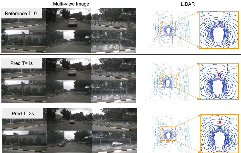
Figure 5: The visualization of Lidar and video predictions.

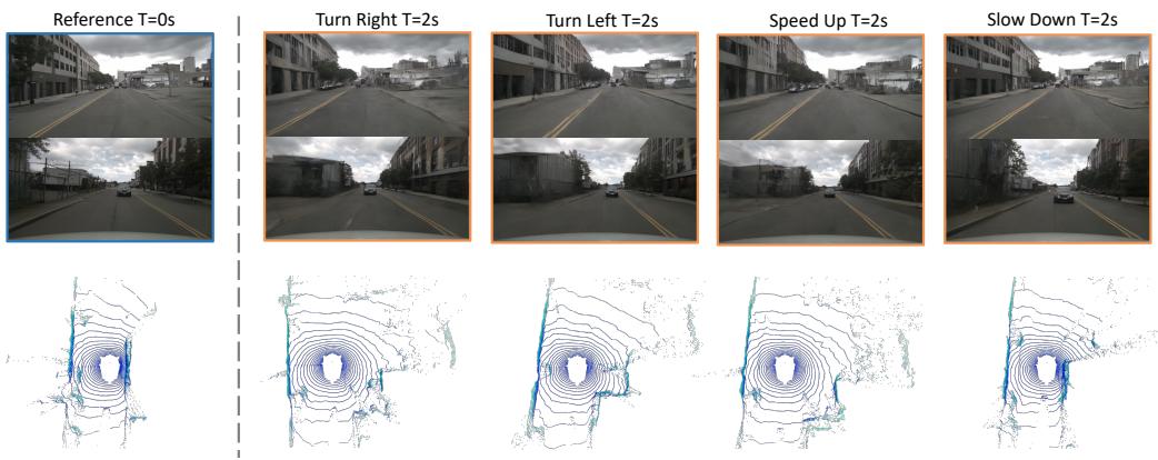
Figure 6: The visualization of controllability. Due to space limitations, we only show the results of the front and rear views for a clearer presentation.

，使其难以用大量未标注数据进行训练。因此我们不将人工注释放作为模型条件。结果如表 4 所示。所提出的方法在不使用人工标注条件的方法中取得了最佳的 FID 和 FVD 性能，并在使用额外条件的方法中表现出可比的结果。激光雷达和视频预测的可视化结果如图5所示。此外，生成过程可由动作条件进行控制。我们将动作代币转换为左转、右转、加速和减速，生成的图像和激光雷达数据可根据这些指令生成。可控性的可视化如图6所示。

Carla. 在 Carla 上的生成质量与在 nuScenes 数据集上的相近，这表明我们的方法在不同数据集间具有可扩展性。视频预测的定量结果见表 4，分别为 36.80（FID 1s）和 43.12（FID 3s）。视频预测的定性结果列于附录。

图5：激光雷达和视频预测的可视化。

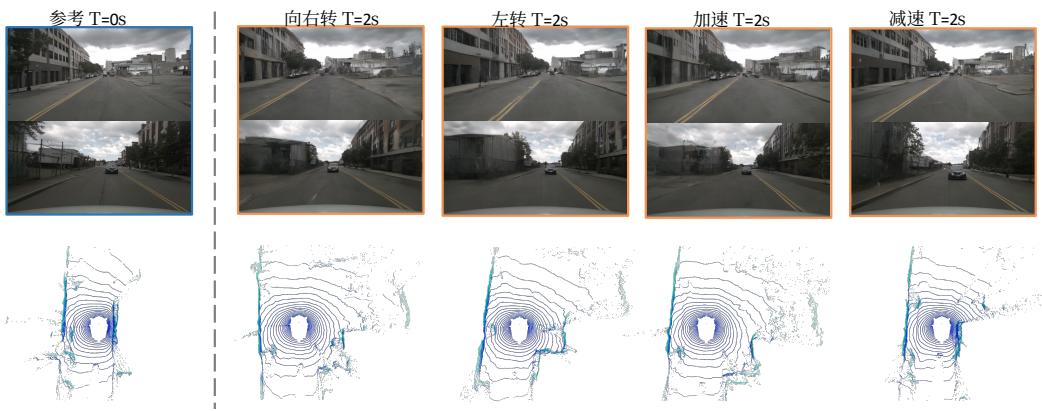
图6：可控性的可视化。由于空间限制，我们仅展示了前视和后视的结果以便更清晰地演示。

5 CONCLUSION

We present BEVWorld, an innovative autonomous driving framework that leverages a unified Bird’s Eye View latent space to construct a multi-modal world model. BEVWorld’s self-supervised learning paradigm allows it to efficiently process extensive unlabeled multimodal sensor data, leading to a holistic comprehension of the driving environment. Furthermore, BEVWorld achieves satisfactory results in multi-modal future predictions with latent diffusion network, showcasing its capabilities through experiments on both real-world(nuScenes) and simulated(carla) datasets. We hope that the work presented in this paper will stimulate and foster future developments in the domain of world models for autonomous driving.

REFERENCES

Andreas Blattmann, Tim Dockhorn, Sumith Kulal, Daniel Mendelevitch, Maciej Kilian, Dominik Lorenz, Yam Levi, Zion English, Vikram Voleti, Adam Letts, et al. Stable video diffusion: Scaling latent video diffusion models to large datasets. arXiv preprint arXiv:2311.15127, 2023.

Daniel Bogdoll, Yitian Yang, and J Marius Zöllner. Muvo: A multimodal generative world model for autonomous driving with geometric representations. arXiv preprint arXiv:2311.11762, 2023.

Tim Brooks, Bill Peebles, Connor Holmes, Will DePue, Yufei Guo, Li Jing, David Schnurr, Joe Taylor, Troy Luhman, Eric Luhman, Clarence $\mathrm{Ng}$ , Ricky Wang, and Aditya Ramesh. Video generation models as world simulators. 2024. URL https://openai.com/research/ video-generation-models-as-world-simulators.

Holger Caesar, Varun Bankiti, Alex H Lang, Sourabh Vora, Venice Erin Liong, Qiang Xu, Anush Krishnan, Yu Pan, Giancarlo Baldan, and Oscar Beijbom. nuscenes: A multimodal dataset for autonomous driving. In Proceedings of the IEEE/CVF conference on computer vision and pattern recognition, pp. 11621–11631, 2020.

Guangyan Chen, Meiling Wang, Yi Yang, Kai Yu, Li Yuan, and Yufeng Yue. Pointgpt: Autoregressively generative pre-training from point clouds. Advances in Neural Information Processing Systems, 36, 2024.

Alexey Dosovitskiy, German Ros, Felipe Codevilla, Antonio Lopez, and Vladlen Koltun. Carla: An open urban driving simulator. In Conference on robot learning, pp. 1–16. PMLR, 2017.

Ruiyuan Gao, Kai Chen, Enze Xie, Lanqing Hong, Zhenguo Li, Dit-Yan Yeung, and Qiang Xu. Magicdrive: Street view generation with diverse 3d geometry control. arXiv preprint arXiv:2310.02601, 2023.

Shenyuan Gao, Jiazhi Yang, Li Chen, Kashyap Chitta, Yihang Qiu, Andreas Geiger, Jun Zhang, and Hongyang Li. Vista: A generalizable driving world model with high fidelity and versatile controllability. 2024.

Ian Goodfellow, Jean Pouget-Abadie, Mehdi Mirza, Bing Xu, David Warde-Farley, Sherjil Ozair, Aaron Courville, and Yoshua Bengio. Generative adversarial networks. Communications of the ACM, 63(11):139–144, 2020.

Xi Guo, Chenjing Ding, Haoxuan Dou, Xin Zhang, Weixuan Tang, and Wei Wu. Infinitydrive: Breaking time limits in driving world models. arXiv preprint arXiv:2412.01522, 2024.

Yingqing He, Tianyu Yang, Yong Zhang, Ying Shan, and Qifeng Chen. Latent video diffusion models for high-fidelity long video generation. arXiv preprint arXiv:2211.13221, 2022.

Jonathan Ho, Tim Salimans, Alexey Gritsenko, William Chan, Mohammad Norouzi, and David J Fleet. Video diffusion models. Advances in Neural Information Processing Systems, 35:8633– 8646, 2022.

Anthony Hu, Gianluca Corrado, Nicolas Griffiths, Zachary Murez, Corina Gurau, Hudson Yeo, Alex Kendall, Roberto Cipolla, and Jamie Shotton. Model-based imitation learning for urban driving. Advances in Neural Information Processing Systems, 35:20703–20716, 2022.

5 结论

我们提出了 BEVWorld，一种创新的自动驾驶框架，利用统一的鸟瞰图潜在空间构建多模态世界模型。BEVWorld 的自监督学习范式使其能够高效处理大量无标签的多模态传感器数据，从而对驾驶环境形成整体理解。此外，BEVWorld 在使用潜在扩散网络进行多模态未来预测方面取得了令人满意的结果，并通过在真实（nuScenes）和仿真（carla）数据集上的实验展示了其能力。我们希望本文的工作能激发并促进自动驾驶领域世界模型的未来发展。

参考文献

Andreas Blattmann, Tim Dockhorn, Sumith Kulal, Daniel Mendelevitch, Maciej Kilian, Dominik Lorenz, Yam Levi, Zion English, Vikram Voleti, Adam Letts, et al. Stable video diffusion: Scaling latent video diffusion models to large datasets. arXiv preprint arXiv:2311.15127, 2023.

Daniel Bogdoll, Yitian Yang, and J Marius Zöllner. Muvo: A multimodal generative world model for autonomous driving with geometric representations. arXiv preprint arXiv:2311.11762, 2023.

Tim Brooks, Bill Peebles, Connor Holmes, Will DePue, Yufei Guo, Li Jing, David Schnurr, Joe Taylor, Troy Luhman, Eric Luhman, Clarence $\mathrm{Ng}$ , Ricky Wang, and Aditya Ramesh. Video generation models as world simulators. 2024. URL https://openai.com/research/ video-generation-models-as-world-simulators.

Holger Caesar, Varun Bankiti, Alex H Lang, Sourabh Vora, Venice Erin Liong, Qiang Xu, Anush Krishnan, Yu Pan, Giancarlo Baldan, and Oscar Beijbom. nuscenes: A multimodal dataset for autonomous driving. In Proceedings of the IEEE/CVF conference on computer vision and pattern recognition, pp. 11621–11631, 2020.

Guangyan Chen, Meiling Wang, Yi Yang, Kai Yu, Li Yuan, and Yufeng Yue. Pointgpt: Autoregressively generative pre-training from point clouds. Advances in Neural Information Processing Systems, 36, 2024.

Alexey Dosovitskiy, German Ros, Felipe Codevilla, Antonio Lopez, and Vladlen Koltun. Carla: An open urban driving simulator. In Conference on robot learning, pp. 1–16. PMLR, 2017.

Ruiyuan Gao, Kai Chen, Enze Xie, Lanqing Hong, Zhenguo Li, Dit-Yan Yeung, and Qiang Xu. Magicdrive: Street view generation with diverse 3d geometry control. arXiv preprint arXiv:2310.02601, 2023.

Shenyuan Gao, Jiazhi Yang, Li Chen, Kashyap Chitta, Yihang Qiu, Andreas Geiger, Jun Zhang, and Hongyang Li. Vista: A generalizable driving world model with high fidelity and versatile controllability. 2024.

Ian Goodfellow, Jean Pouget-Abadie, Mehdi Mirza, Bing Xu, David Warde-Farley, Sherjil Ozair, Aaron Courville, and Yoshua Bengio. Generative adversarial networks. Communications of the ACM, 63(11):139–144, 2020.

Xi Guo, Chenjing Ding, Haoxuan Dou, Xin Zhang, Weixuan Tang, and Wei Wu. Infinitydrive: Breaking time limits in driving world models. arXiv preprint arXiv:2412.01522, 2024.

Yingqing He, Tianyu Yang, Yong Zhang, Ying Shan, and Qifeng Chen. Latent video diffusion models for high-fidelity long video generation. arXiv preprint arXiv:2211.13221, 2022.

Jonathan Ho, Tim Salimans, Alexey Gritsenko, William Chan, Mohammad Norouzi, and David J Fleet. Video diffusion models. Advances in Neural Information Processing Systems, 35:8633– 8646, 2022.

Anthony Hu, Gianluca Corrado, Nicolas Griffiths, Zachary Murez, Corina Gurau, Hudson Yeo, Alex Kendall, Roberto Cipolla, and Jamie Shotton. Model-based imitation learning for urban driving. Advances in Neural Information Processing Systems, 35:20703–20716, 2022.

APPENDIX

A QUALITATIVE RESULTS

In this section, qualitative results are presented to demonstrate the performance of the proposed method.

A.1 TOKENIZER RECONSTRUCTIONS

The visualization of tokenizer reconstructions are shown in Figure 7 and Figure 8. The proposed tokenizer can recover the image and Lidar with the unified BEV features.

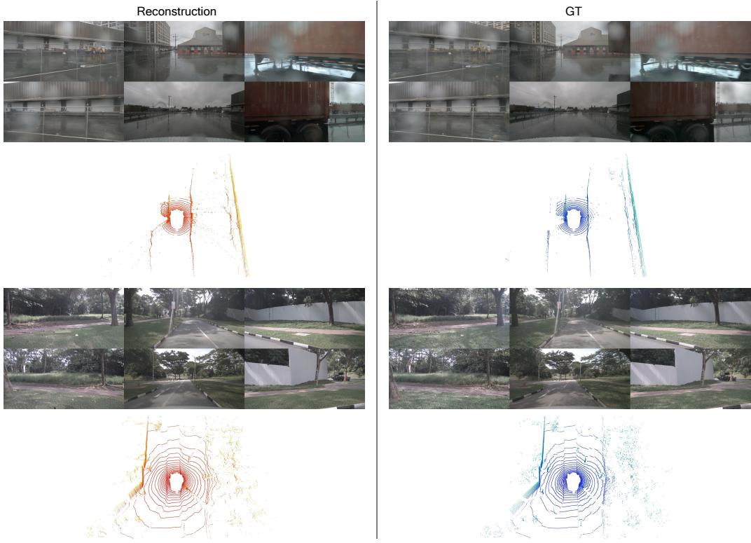
Figure 7: The visualization of LiDAR and video reconstructions on nuScenes dataset.

A.2 MULTI-MODAL FUTURE PREDICTIONS

Diverse generation. The proposed diffusion-based world model can produce high-quality future predictions with different driving conditions, and both the dynamic and static objects can be generated properly. The qualitative results are illustrated in Figure 9 and Figure 10.

Controllability. We present more visual results of controllability in Figure 11. The generated images and Lidar exhibit a high degree of consistency with action, which demonstrates that our world model has the potential of being a simulator.

PSNR metric. PSNR metric has the problem of being unable to differentiate between blurring and sharpening. As shown in Figure 12, the image quality of L & C is better the that of C, while the psnr metric of L & C is worse than that of C.

B IMPLEMENTATION DETAILS

Training details of tokenizer. We trained our model using 32 GPUs, with a batch size of 1 per card. We used the AdamW optimizer with a learning rate of 5e-4, beta ${}_{=0.5}$ , and beta $2=0.9$ , following a

附录

A 定性结果

在本节中，展示了定性结果以证明所提方法的性能。

A.1 分词器重建

代币器重建的可视化结果如图7和图8所示。所提出的代币器能够利用统一的 BEV 特征重建图像和激光雷达。

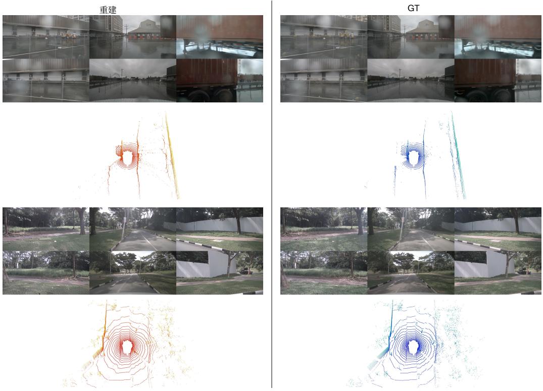
图7：在 nuScenes 数据集上激光雷达和视频重建的可视化。

A.2 多模态未来预测

多样化生成。 所提出的基于扩散的世界模型能够在不同驾驶条件下生成高质量的未来预测，动态和静态物体都能被恰当地生成。定性结果在图9和图10中展示。

可控性。我们在图11中给出更多有关可控性的可视化结果。生成的图像和激光雷达与动作高度一致，说明我们的世界模型具有成为模拟器的潜力。

PSNR 指标。 PSNR 指标无法区分模糊与锐化。如图12所示，L 与 C 的图像质量优于 C，但 L 与 C 的 PSNR 指标却比 C 更差。

B 实现细节

分词器的训练细节。我们使用 32 张 GPU 训练模型，每张卡的批量大小为 1。我们使用 AdamW 优化器，学习率为5e‑4，beta ${}_{.=0.5}$ ，和beta $2=0.9$ ，遵循 a

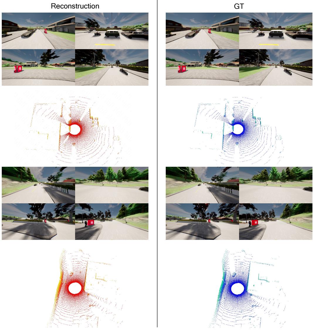
Figure 8: The visualization of LiDAR and video reconstructions on Carla dataset.

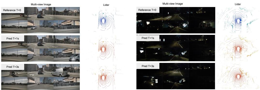
Figure 9: The visualization of LiDAR and future predictions on nuScenes dataset.

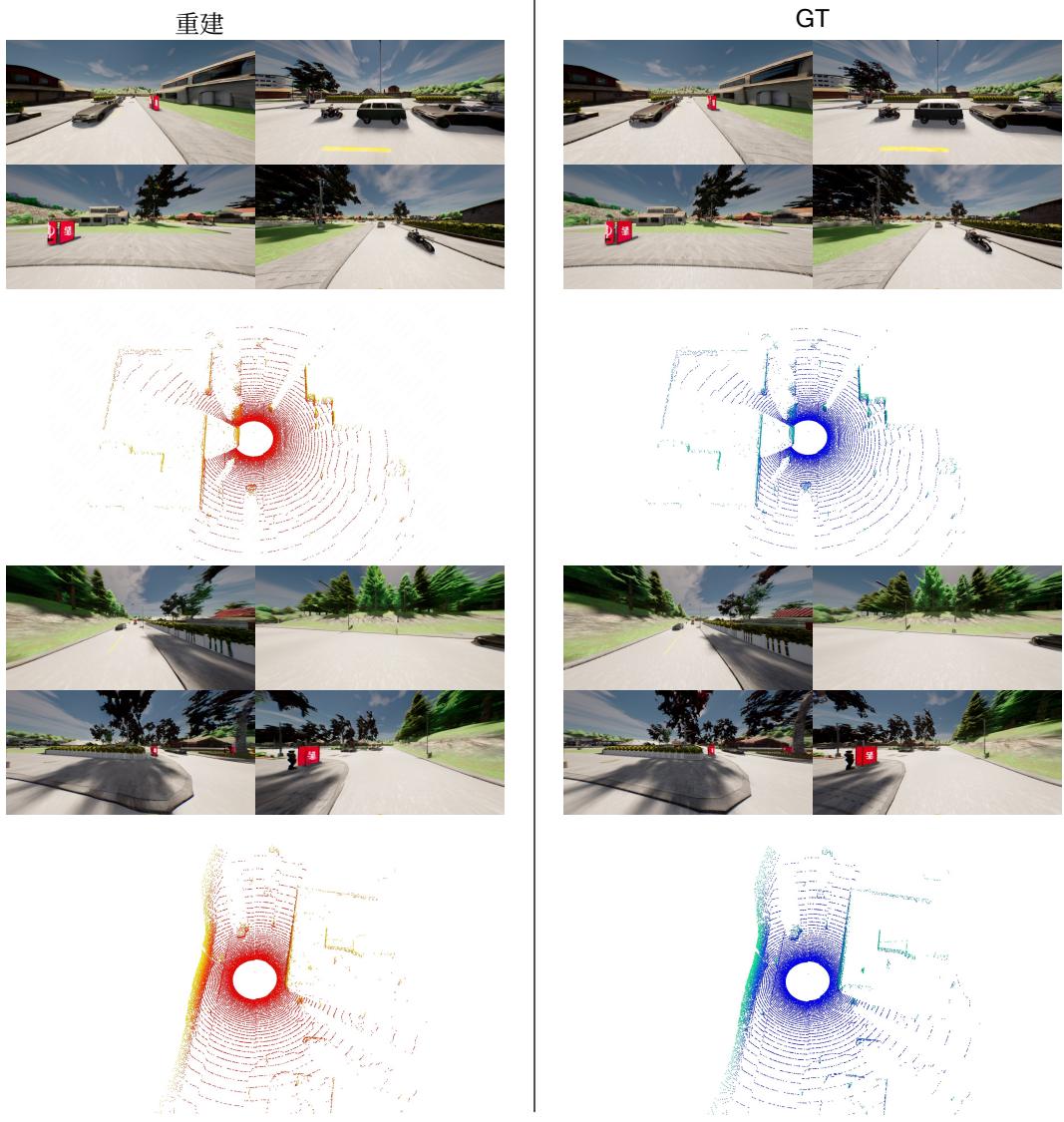
图8：在 Carla 数据集上对激光雷达和视频重建的可视化。

图9：在 nuScenes 数据集上对激光雷达和未来预测的可视化。

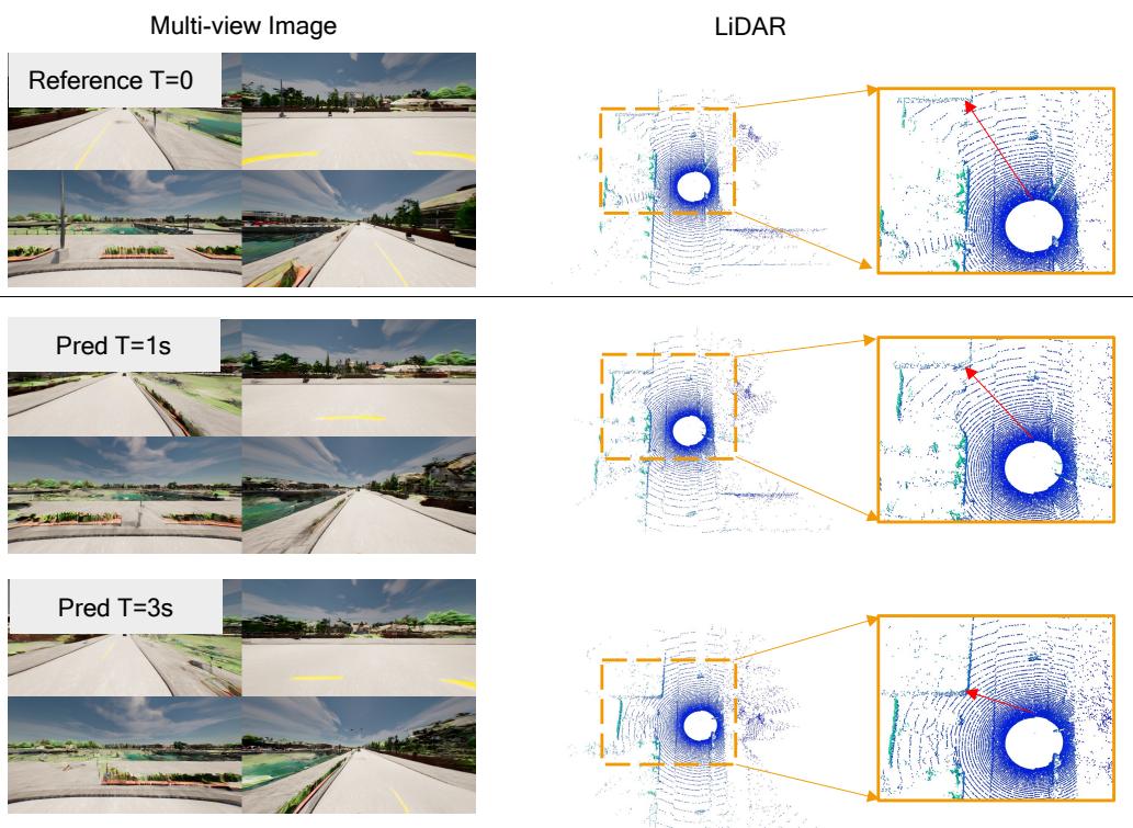
Figure 10: The visualization of LiDAR and future predictions on Carla dataset.

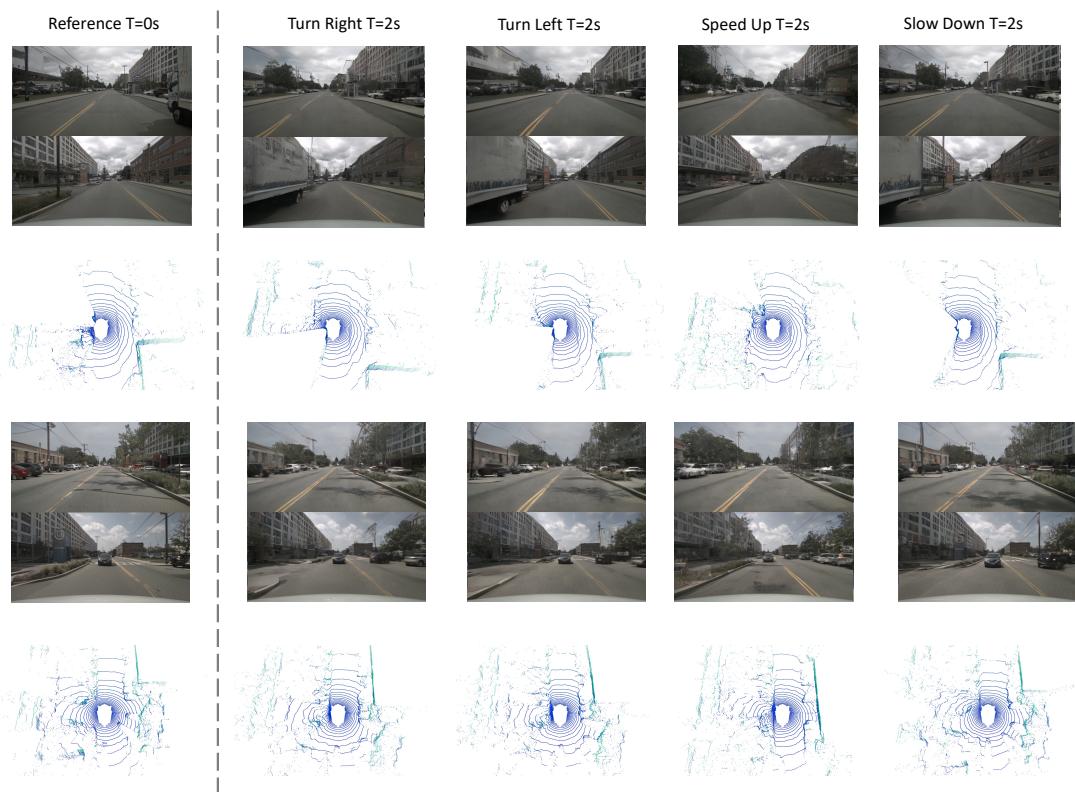
Figure 11: More visual results of controllability.

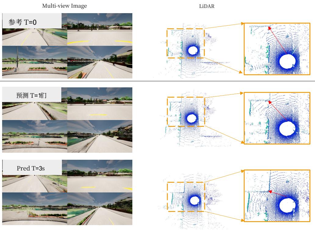
图10：LiD 和未来预测在 Carla 数据集上的可视化。

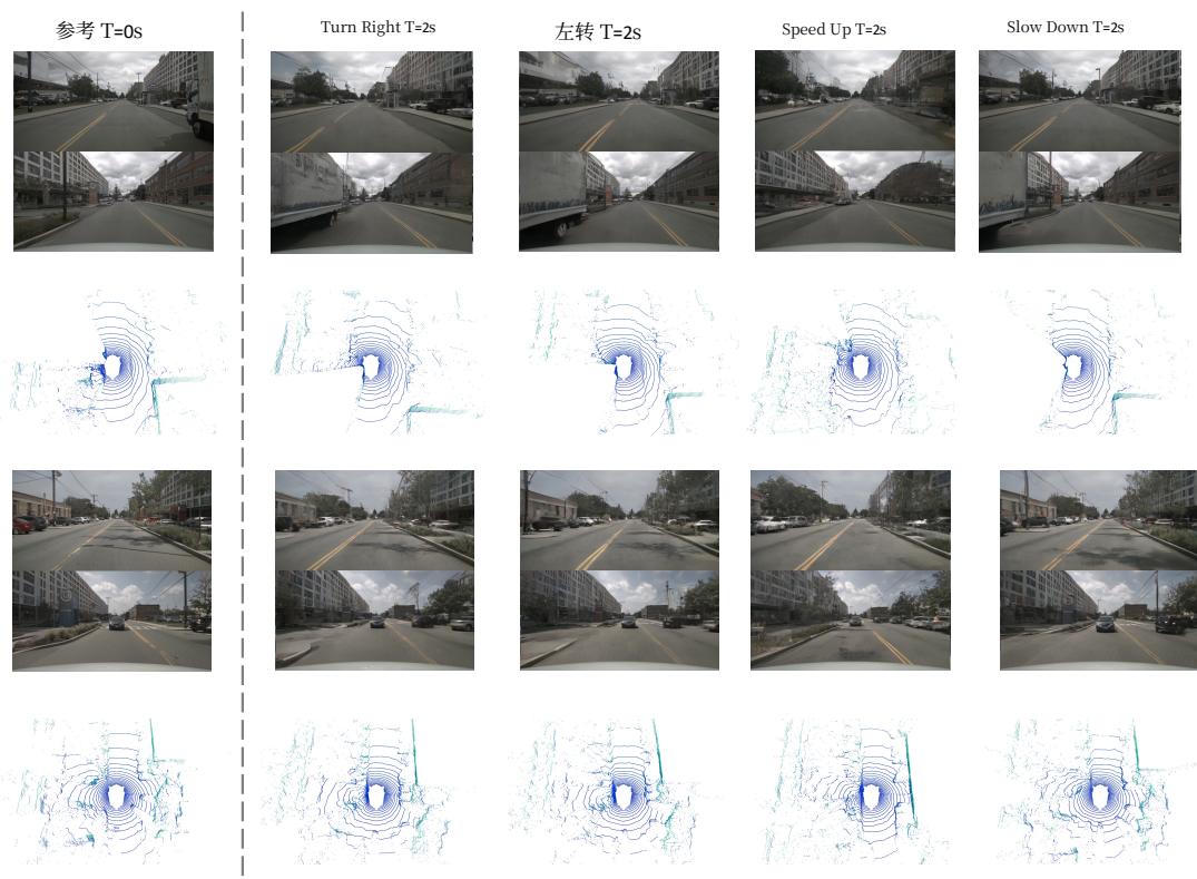
图11：更多关于可控性的可视化结果。

Figure 12: The visualization of C and L & C.

cosine learning rate decay strategy. The multi-task loss function includes a perceptual loss weight of 0.1, a lidar loss weight of 1.0, and an RGB L1 reconstruction loss weight of 1.0. For the GAN training, we employed a warm-up strategy, introducing the GAN loss after 30,000 iterations. The discriminator loss weight was set to 1.0, and the generator loss weight was set to 0.1.

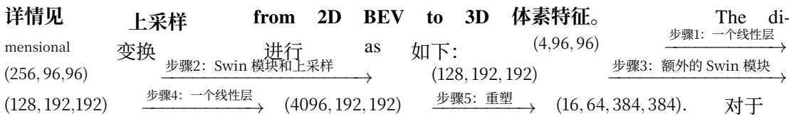
Details on Upsampling from 2D BEV to 3D Voxel Features. The dimensional transformation proceeds as follows: (4, 96, 96) Step1: a linear layer (256, 96, 96) Step2: Swin Blocks and upsampling (128, 192, 192) Step3: additional Swin Blocks (128, 192, 192) Step4: a linear layer (4096, 192, 192) Step5: reshaping−−−−−−−−→ (16, 64, 384, 384). For the upsampling in Step 2, we adopt Patch Expanding, which is commonly used in ViT-based approaches and can be seen as the reverse operation of Patch Merging. The linear layer in Step 4 predicts a local region of shape (16, 64, $r_y,r_x)$ ), where spatial sizes are adjusted (e.g., $r_y=2$ , $r_x=2$ ), followed by reshaping in Step 5 to the final 3D feature shape.

Composition of 3D Voxel Features. Along each ray, we perform uniform sampling, and the depth t of the sampled points is a predefined value, not predicted by the model. The feature ${\mathbf{v}}_{\mathrm{i}}$ at these sampled points is obtained through linear interpolation, while the blending weight w is predicted from the sampled features ${\mathbf{v}}_{\mathrm{i}}$ (as described in Equation 1). This is a standard differentiable rendering process.

C BROADER IMPACTS

The concept of a world model holds significant relevance and diverse applications within the realm of autonomous driving. It serves as a versatile tool, functioning as a simulator, a generator of long-tail data, and a pre-trained model for subsequent tasks. Our proposed method introduces a multi-modal BEV world model framework, designed to align seamlessly with the multi-sensor configurations inherent in existing autonomous driving models. Consequently, integrating our approach into current autonomous driving methodologies stands to yield substantial benefits.

D LIMITATIONS

It is widely acknowledged that inferring diffusion models typically demands around 50 steps to attain denoising results, a process characterized by its sluggishness and computational expense. Regrettably, we encounter similar challenges. As pioneers in the exploration of constructing a multi-modal world model, our primary emphasis lies on the generation quality within driving scenes, prioritizing it over computational overhead. Recognizing the significance of efficiency, we identify the adoption of onestep diffusion as a crucial direction for future improvement in the proposed method. Regarding the quality of the generated imagery, we have noticed that dynamic objects within the images sometimes suffer from blurriness. To address this and further improve their clarity and consistency, a dedicated module specifically tailored for dynamic objects may be necessary in the future.

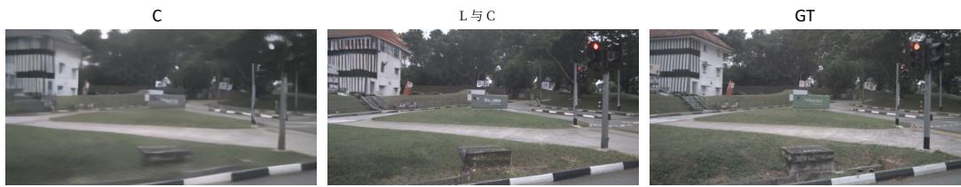
图12：C 与 L 与 C 的可视化。

余弦学习率衰减策略。多任务损失函数包括感知损失权重为0.1、激光雷达损失权重为1.0以及RGB L1重建损失权重为1.0。在生成对抗网络训练中，我们采用了预热策略，在30,000次迭代后引入生成对抗网络损失。判别器损失权重设置为1.0，生成器损失权重设置为 $0.1_{\circ }$ 步骤2中的上采样，我们采用 Patch Expanding，这在基于 ViT 的方法中很常见并且可以看作是 Patch Merging 的逆操作。步骤4中的线性层预测形状为 (16, 64, $r_y,r_x)$ 的局部区域，其中空间尺寸会被调整（例如 $r_y=2$ , $r_x=2,$ ），随后在步骤5中重塑为最终的三维特征形状。

3D 体素特征的组成。沿着每条光线，我们进行均匀采样，采样点的深度 t 为预定义值，并非由模型预测。在这些采样点处的特征 ${\mathbf{v}}_{\mathrm{i}}$ 通过线性插值获得，而混合权重 w 则由采样到的特征 ${\mathbf{v}}_{\mathrm{i}}$ 预测（如公式 1 所述）。这是一个标准的可微渲染过程。

C 更广泛的影响

世界模型的概念在自动驾驶领域具有重要意义和多样化的应用。它可以作为模拟器、生成长尾数据的工具，以及用于后续任务的预训练模型。我们提出的方法引入了一个多模态BEV 世界模型框架，旨在与现有自动驾驶模型中固有的多传感器配置无缝对齐。因此，将我们的方法整合到当前的自动驾驶方法中，有望带来显著收益。

D 局限性

众所周知，推理扩散模型通常需要约 50 步才能达到去噪效果，这是一个缓慢且计算开销大的过程。不幸的是，我们也面临类似挑战。作为构建多模态世界模型探索的先驱者，我们的主要关注点在于驾驶场景下的生成质量，优先于计算开销。鉴于效率的重要性，我们认为在所提方法中采用一步扩散是未来改进的关键方向。关于生成图像的质量，我们注意到图像中的动态物体有时会出现模糊。为了解决这一问题并进一步提升其清晰度与一致性，未来可能需要专门针对动态物体的模块。