Driving in the Occupancy World: Vision-Centric 4D Occupancy Forecasting and Planning via World Models for Autonomous Driving

Yu Yang 1*, Jianbiao Mei 1*, Yukai Ma 1, Siliang $\mathbf{D}{\mathbf{u}}^{2†}$ , Wenqing Chen 2, Yijie Qian 1, Yuxiang Feng 1, Yong Liu 1†

1Zhejiang University 2Huawei Technologies
{yu.yang, jianbiaomei, yukaima, yijieqian, yuxiangfeng}@zju.edu.cn
{dusiliang, chenwenqing7}@huawei.com,yongliu $@$ iipc.zju.edu.cn Project Page: https://drive-occworld.github.io/

Abstract

World models envision potential future states based on various ego actions. They embed extensive knowledge about the driving environment, facilitating safe and scalable autonomous driving. Most existing methods primarily focus on either data generation or the pretraining paradigms of world models. Unlike the aforementioned prior works, we propose Drive-OccWorld, which adapts a vision-centric 4D forecasting world model to end-to-end planning for autonomous driving. Specifically, we first introduce a semantic and motionconditional normalization in the memory module, which accumulates semantic and dynamic information from historical BEV embeddings. These BEV features are then conveyed to the world decoder for future occupancy and flow forecasting, considering both geometry and spatiotemporal modeling. Additionally, we propose injecting flexible action conditions, such as velocity, steering angle, trajectory, and commands, into the world model to enable controllable generation and facilitate a broader range of downstream applications. Furthermore, we explore integrating the generative capabilities of the 4D world model with end-to-end planning, enabling continuous forecasting of future states and the selection of optimal trajectories using an occupancy-based cost function. Comprehensive experiments conducted on the nuScenes, nuScenes-Occupancy, and Lyft-Level5 datasets illustrate that our method can generate plausible and controllable 4D occupancy, paving the way for advancements in driving world generation and end-to-end planning.

On the other hand, to embed world knowledge and simulate the real-world physics of the driving environment, recent works (Zhang et al. 2023b; Min et al. 2024; Yang et al. 2024b) have introduced the world model (Ha and Schmidhuber 2018) to facilitate scalable autonomous driving. Nevertheless, most of them primarily focus on either data generation or the pretraining paradigms of world models, neglecting the enhancement of safety and robustness for end-to-end planning. For example, many studies (Ma et al. $2024\mathrm{a}$ ; Wang et al. 2023b; Hu et al. 2023a) aimed to generate high-fidelity driving videos through world models to provide additional data for downstream training. The very recent ViDAR (Yang et al. 2024b) pre-trained the visual encoder by forecasting point clouds from historical visual input, enhancing performance on downstream tasks such as vision-centric 3D detection and segmentation. Therefore, we believe that integrating the future forecasting capabilities of world models with endto-end planning remains a worthwhile area for exploration.

In this work, we investigate 4D forecasting and planning using world models to implement future state prediction and end-to-end planning. With the capability to envision various futures based on different ego actions, a world model allows the agent to anticipate potential outcomes in advance. As illustrated in Figure 1, the world model predicts the future state of the environment under different action conditions, using historical observations and various ego actions. Subsequently, the planner employs a cost function that considers both safety and the 3D structure of the environment to select the most suitable trajectory, enabling the agent to navigate effectively in diverse situations. Finally, the predicted future state and selected optimal trajectory can be reintroduced into the world model for the next rollout, facilitating continuous future prediction and trajectory planning. We experimentally demonstrate that leveraging the future forecasting capability of world models enhances the planner’s generalization and safety robustness while providing more explainable decision-making, as detailed in Section 4.

1 Introduction

Autonomous driving (AD) algorithms have advanced significantly in recent decades (Ayoub et al. 2019; Chen et al. 2023). These advancements have transitioned from modular pipelines (Guo et al. 2023; Li et al. 2023b) to end-to-end models (Hu et al. 2023b; Jiang et al. 2023), which plan trajectories directly from raw sensor data in a unified pipeline. However, due to insufficient world knowledge for forecasting dynamic environments, these methods exhibit deficiencies in generalization ability and safety robustness.

Specifically, we propose Drive-OccWorld, a visioncentric 4D forecasting and planning world model for autonomous driving. Our Drive-OccWorld exhibits three key features: (1) Understanding how the world evolves through 4D occupancy forecasting. Drive-OccWorld predicts plau

在 OccupancyWorld 中驾驶：通过用于自动驾驶的世界模型进行以视觉为中心的四维占用预测与规划

Yu Yang 1*，Jianbiao Mei ${}^{1\ast }$ ，Yukai Ma 1，Siliang Du 2 †， Wenqing Chen 2，Yijie Qian 1，Yuxiang Feng 1, Yong Liu 1†

1浙江大学2华为技术有限公司
{yu.yang, jianbiaomei,yukaima,yijieqian,yuxiangfeng}@zju.edu.cn{
dusiliang, chenwenqing7}@huawei.com,yongliu@iipc.zju.edu.cn 项

目页面: https://drive-occworld.github.io/

摘要

世界模型根据不同的自车动作设想潜在的未来状态。它们蕴含关于驾驶环境的大量知识，有助于实现安全且可扩展的自动驾驶。大多数现有方法主要关注世界模型的数据生成或预训练范式。与上述先前工作不同，我们提出了Drive-OccWorld，将以视觉为中心的四维预测世界模型适配到用于自动驾驶的端到端规划。具体而言，我们首先在记忆模块中引入了语义和运动条件归一化，该模块从历史BEV嵌入中累积语义和动态信息。随后，这些BEV特征被传递到世界解码器，用于未来占用和流动的预测，同时兼顾几何与时空建模。此外，我们提出将灵活的动作条件（如速度、转向角、轨迹和指令）注入世界模型，以实现可控生成并促进更广泛的下游应用。进一步地，我们探索将四维世界模型的生成能力与端到端规划相结合，实现未来状态的连续预测，并使用基于占用的代价函数选择最优轨迹。在 nuScenes、nuScenes‑Occupancy 和 Lyft‑Level5 数据集上进行的全面实验表明，我们的方法能够生成合理且可控的四维占用，为驾驶世界生成和端到端规划的进步铺平了道路。

另一方面，为了嵌入世界知识并模拟驾驶环境的真实物理，近期工作（Zhang 等人 2023b；Min 等人 2024；Yang 等人 2024b）引入了世界模型（Ha 和Schmidhuber 2018）以促进可扩展的自动驾驶。然而，它们中的大多数主要关注世界模型的数据生成或预训练范式，忽视了增强端到端规划的安全性和鲁棒性。例如，许多研究（Ma 等人 2024a；Wang 等人 2023b；Hu 等人2023a）旨在通过世界模型生成高保真度的驾驶视频，为下游训练提供额外数据。最新的 ViDAR（Yang 等人2024b）通过从历史视觉输入预测点云来对视觉编码器进行预训练，从而提升了在以视觉为中心的 3D 检测和分割等下游任务上的表现。因此，我们认为将世界模型的未来预测能力与端到端规划相结合仍然是一个值得探索的方向。

在本工作中，我们使用世界模型研究 4D 预测和规划，以实现未来状态预测和端到端规划。世界模型具备基于不同自车动作构想多种未来的能力，使智能体能够提前预见潜在结果。如图 1 所示，世界模型使用历史观测和多种自车动作，预测在不同动作条件下环境的未来状态。随后，规划器采用同时考虑安全性和环境三维结构的代价函数来选择最合适的轨迹，从而使智能体在各种情形中有效导航。最终，预测的未来状态和选定的最优轨迹可以重新引入世界模型以进行下一次展开，促进连续的未来预测和轨迹规划。我们通过实验展示，利用世界模型的未来预测能力能够提升规划器的泛化和安全鲁棒性，同时提供更具可解释性的决策，如第4节所述。

1 引言

自动驾驶(AD)算法在近几十年里取得了显著进展（Ayoub 等人 2019；Chen 等人 2023）。这些进展已经从模块化流程（Guo 等人 2023；Li 等人 2023b）转向端到端模型（Hu 等人 2023b；Jiang 等人 2023），这些模型在统一的流程中直接从原始传感器数据规划轨迹。然而，由于用于预测动态环境的世界知识不足，这些方法在泛化能力和安全鲁棒性方面存在不足。

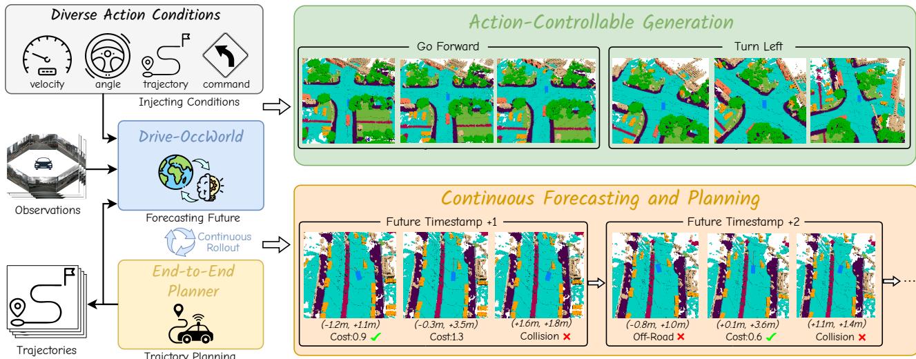
Figure 1: 4D Occupancy Forecasting and Planning via World Model. Drive-OccWorld takes observations and trajectories as input, incorporating flexible action conditions for action-controllable generation. By leveraging world knowledge and the generative capacity of the world model, we further integrate it with a planner for continuous forecasting and planning.

sible future states based on accumulated historical experiences. It comprises three key components: a history encoder that encodes multi-view geometry BEV embeddings, a memory queue that accumulates historical information, and a future decoder that forecasts occupancy and flows through spatiotemporal modeling. Additionally, we introduce a semantic- and motion-conditional normalization to aggregate significant features. (2) Generating various future states based on action conditions. We incorporate a flexible set of action conditions (e.g., velocity, steering angle, trajectory, and high-level commands), which are encoded and injected into the world decoder through a unified interface, empowering the world model’s capability for actioncontrollable generation. (3) Planning trajectories with the world model. Since the world model can forecast future occupancy and flow, providing perception and prediction results that include the fine-grained states of both agents and background elements, we further design a planner to select the optimal trajectory based on a comprehensive occupancybased cost function.

We evaluate Drive-OccWorld using the nuScenes, nuScenes-Occupancy, and Lyft-Level5 datasets. It outperforms previous methods by $9.5\%$ in ${\mathrm{mIoU}}_f$ and $5.1\%$ i n ${\mathrm{VPQ}}_f$ on nuScenes, by $6.1\%$ in ${\mathrm{mIoU}}_f$ and $5.2\%$ in ${\mathrm{VPQ}}_f$ on Lyft-Level5 for forecasting the inflated occupancy of movable objects and their 3D backward centripetal flow. On the nuScenes-Occupancy benchmark, it achieves a $4.3\%$ improvement in fine-grained occupancy forecasting. Additionally, experiments on trajectory planning indicate that DriveOccWorld is effective for safe motion planning.

Our main contributions can be summarized as follows:

• We propose Drive-OccWorld, a vision-centric world model designed for forecasting 4D occupancy and dynamic flow, achieving new state-of-the-art performance on both the nuScenes and Lyft benchmarks. • We develop a simple yet efficient semantic- and motionconditional normalization module for semantic enhancement and motion compensation, which improves forecasting and planning performance.

• We incorporate flexible action conditions into DriveOccWorld to enable action-controllable generation and explore integrating the world model with an occupancybased planner for continuous forecasting and planning.

2 Related Works

2.1 World Models for Autonomous Driving

Existing world models for autonomous driving can be primarily classified into 2D image-based and 3D volume-based models, based on the generation modality of future states.

2D Image-based Models aim to predict future driving videos using reference images and other conditions (e.g., actions, HDMaps, 3D boxes, and text prompts). GAIA-1 (Hu et al. 2023a) uses an autoregressive transformer as a world model to predict future image tokens based on past image, text, and action tokens. Other methods, such as DriveDreamer (Wang et al. 2023b), ADriver-I (Jia et al. 2023), DrivingDiffusion (Li, Zhang, and Ye 2023), GenAD (Yang et al. 2024a), Vista (Gao et al. 2024), Delphi (Ma et al. 2024a), and Drive-WM (Wang et al. 2024b), use latent diffusion models (LDMs) (Rombach et al. 2022; Blattmann et al. 2023) for image-to-driving video generation. These methods focus on designing modules to incorporate actions, BEV layouts, and other priors into the denoising process, resulting in more coherent and plausible future video generations.

3D Volume-based Models forecast future states in the form of point clouds or occupancy. Copilot4D (Zhang et al. 2023b) tokenizes LiDAR observations with VQVAE (Van Den Oord, Vinyals et al. 2017) and predicts future point clouds via discrete diffusion. ViDAR (Yang et al. 2024b) implements a visual point cloud forecasting task to pre-train visual encoders. UnO (Agro et al. 2024) forecasts a continuous

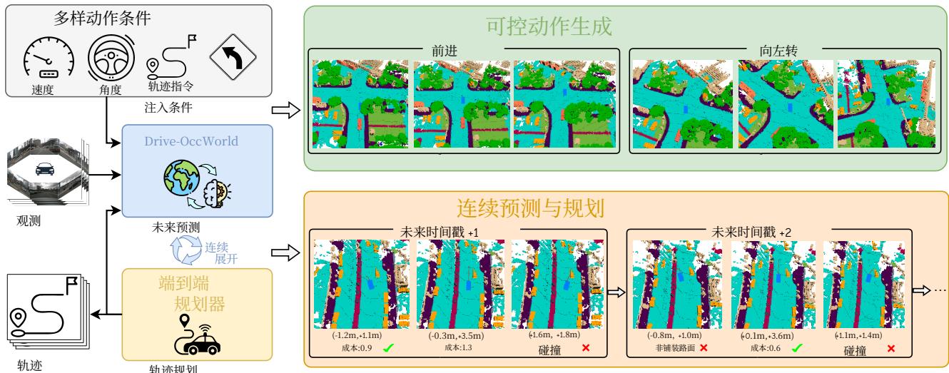
图 1:通过世界模型进行四维占用预测与规划。Drive‑OccWorld 以观测和轨迹为输入，结合灵活的动作条件以实现可控动作生成。通过利用世界知识和世界模型的生成能力，我们进一步将其与规划器整合用于连续预测与规划。

它由三部分组成：一个编码多视角几何 BEV 嵌入的历史编码器、一个累积历史信息的记忆队列，以及一个通过时空建模来预测占用和流场的未来解码器。此外，我们引入了语义与运动条件归一化以聚合重要特征。(2)基于动作条件生成多样的未来状态。我们整合了一组灵活的动作条件（例如，速度、转向角、轨迹和高层指令），将其编码后通过统一接口注入到世界解码器，从而赋予世界模型可受动作控制的生成能力。(3)使用世界模型进行轨迹规划。由于世界模型能够预测未来占用和流场，提供包含智能体与背景要素细粒度状态的感知与预测结果，我们进一步设计了一个规划器，基于综合的占用基代价函数选择最优轨迹。

我们在 nuScenes、nuScenes‑Occupancy 和Lyft‑Level5 数据集上评估 Drive‑OccWorld。在 nuScenes 上，它在 mIoUf 上比之前的方法提高了 $9.5\%$ ，在 VPQf 上提高了$5.1\%$ ；在 Lyft‑Level5 上，针对可移动物体的膨胀占据及其三维反向向心流的预测，mIoUf 提高了 $6.1\%$ ，VPQf 提高了 5.2${\%}_{>}$ 。在 nuScenes‑Occupancy 基准上，它在细粒度占据预测方面取得了 $4.3\%$ 的提升。此外，轨迹规划实验表明Drive‑OccWorld 对安全运动规划是有效的。

我们的主要贡献可总结如下：

•我们提出了 Drive‑OccWorld，一种以视觉为中心的世界模型，旨在预测 4D 占据 和动态流，在nuScenes 和 Lyft 基准上实现了新的最先进性能。

• 我们开发了一个简单而高效的语义与运动条件归一化模块，用于语义增强

和运动补偿，从而提升了预测与规划性能。

•我们在 Drive‑OccWorld 中引入了灵活的动作条件，以实现可控动作生成，并探索将该世界模型与基于占用的规划器相结合，用于连续预测与规划。

2 相关工作

2.1 自动驾驶的世界模型

现有用于自动驾驶的世界模型，按未来状态的生成模态，主要可分为基于2D图像和基于3D体积的模型。

2D 图像类模型 旨在使用参考图像和其他条件（例如，动作、HDMaps、3D 包围盒和文本提示）来预测未来的驾驶视频。GAIA‑1 (Hu 等人 2023a) 使用一个自回归变换器作为世界模型，根据过去的图像、文本和动作令牌预测未来的图像令牌。其他方法，例如 Drive‑Dreamer (Wang 等人 2023b)、ADriver‑I(Jia 等人 2023)、DrivingDiffusion (Li, Zhang, and Ye2023)、GenAD (Yang 等人 2024a)、Vista (Gao 等人 2024)、Delphi (Ma 等人 2024a) 和 Drive‑WM (Wang 等人 2024b)，使用LDMs（潜在扩散模型）(Rombach et al. 2022;Blattmann et al. 2023) 进行图像到驾驶视频的生成。这些方法侧重于设计模块以在去噪过程中融合动作、BEV 布局及其他先验，从而产生更连贯且更可信的未来视频生成。

3DVolume-basedModels 以点云或占用的形式预测未来状态。Copilot4D (Zhang et al. 2023b) 使用 VQVAE (Van DenOord, Vinyals et al. 2017) 对 LiDAR 观测进行分词，并通过离散扩散预测未来点云。ViDAR (Yang et al. 2024b) 实现了一个视觉点云预测任务来对视觉编码器进行预训练。UnO (Agro et al. 2024) 预测一个连续的

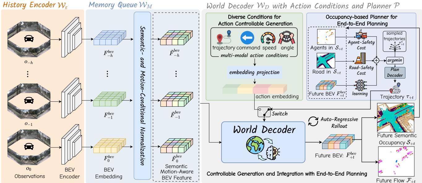
Figure 2: Overview of Drive-OccWorld. (a) The history encoder extracts multi-view image features and transforms them into BEV embeddings. (b) The memory queue employs semantic- and motion-conditional normalization to aggregate historical information. © The world decoder incorporates action conditions to generate various future occupancies and flows. Integrating the world decoder with an occupancy-based planner enables continuous forecasting and planning.

occupancy field with self-supervision from LiDAR data. OccWorld (Zheng et al. 2023) and OccSora (Wang et al. 2024a) compact the occupancy input with a scene tokenizer and use a generative transformer to predict future occupancy. UniWorld (Min et al. 2023) and DriveWorld (Min et al. 2024) propose 4D pre-training via 4D occupancy reconstruction.

In this work, we investigate potential applications of the world model by injecting action conditions to enable actioncontrollable generation and integrating this generative capability with end-to-end planners for safe driving.

3 Method

3.1 Preliminary

An end-to-end autonomous driving model aims to control a vehicle (i.e., plan trajectories) directly based on sensor inputs and ego actions ( $\mathrm{Hu}$ et al. 2023b). Formally, given historical sensor observations {o−h,…,o−1,o0}\{ o _ { - h } , \ldots , o _ { - 1 } , o _ { 0 } \}{o−h​,…,o−1​,o0​} and ego trajectories {τ−h,…,τ−1,τ0}\{ \tau _ { - h } , \ldots , \tau _ { - 1 } , \tau _ { 0 } \}{τ−h​,…,τ−1​,τ0​} over $h$ timestamps, an end-toend model $\mathcal{A}$ predicts desirable ego trajectories {τ1,…,τf}\{ \tau _ { 1 } , \ldots , \tau _ { f } \}{τ1​,…,τf​} for the future $f$ timestamps:

A({o−h,…,o−1,o0},{τ−h,…,τ−1,τ0})={τ1,…,τf} A ( \{ o _ { - h } , \ldots , o _ { - 1 } , o _ { 0 } \} , \{ \tau _ { - h } , \ldots , \tau _ { - 1 } , \tau _ { 0 } \} ) = \{ \tau _ { 1 } , \ldots , \tau _ { f } \} A({o−h​,…,o−1​,o0​},{τ−h​,…,τ−1​,τ0​})={τ1​,…,τf​}

A driving world model $\mathcal{W}$ can be viewed as a generative model that takes prior observations and ego actions {a−h,…,a−1,a0}\{ a _ { - h } , \dotsc , a _ { - 1 } , a _ { 0 } \}{a−h​,…,a−1​,a0​} as input, generating plausible future states {s1,…,sf}\{ s _ { 1 } , \ldots , s _ { f } \}{s1​,…,sf​} of the environment:

W({o−h,…,o−1,o0},{a−h,…,a−1,a0})={s1,…,sf} { \mathcal { W } } ( \{ o _ { - h } , \ldots , o _ { - 1 } , o _ { 0 } \} , \{ a _ { - h } , \ldots , a _ { - 1 } , a _ { 0 } \} ) = \{ s _ { 1 } , \ldots , s _ { f } \} W({o−h​,…,o−1​,o0​},{a−h​,…,a−1​,a0​})={s1​,…,sf​}

where ego actions $a$ can be injected into the controllable generation process in various forms, i.e., velocity, steering angle, ego trajectory, and high-level commands.

Given the world model’s ability to foresee future states, we propose integrating it with a planner to fully exploit the capabilities of the world model in end-to-end planning. Specifically, we introduce an auto-regressive framework termed Drive-OccWorld, which consists of a generative world model $\mathcal{W}$ to forecast future occupancy and flow states, and an occupancy-based planner $\mathcal{P}$ that employs a cost function to select the optimal trajectory based on evaluating future predictions. Formally, we formulate DriveOccWorld as follows, which auto-regressively predicts the future state and trajectory at the next timestamp:

W({o−h,…,o−1,o0},{s1,…,st−1,st},{a−h,…,a−1,a0,…,at−1,at})=st+1 \begin{array} { c } { { { \mathcal { W } ( \{ o _ { - h } , \ldots , o _ { - 1 } , o _ { 0 } \} , \{ s _ { 1 } , \ldots , s _ { t - 1 } , s _ { t } \} , } } } \\ { { { \{ a _ { - h } , \ldots , a _ { - 1 } , a _ { 0 } , \ldots , a _ { t - 1 } , a _ { t } \} \big ) = s _ { t + 1 } } } } \end{array} W({o−h​,…,o−1​,o0​},{s1​,…,st−1​,st​},{a−h​,…,a−1​,a0​,…,at−1​,at​})=st+1​​

$$\mathcal{P}(f_o(s_{t+1},{\tau }_{t+1}^{\ast }))={\tau }_{t+1}$$

where $f_o$ is the occupancy-based cost function, and ${\tau }_{t+1}^{\ast }$ denotes sampled trajectory proposals at the $t+1$ timestamp.

Notably, for action-controllable generation, $a$ can be injected into $\mathcal{W}$ as conditions in the form of velocity, etc., and $\mathcal{P}$ is discarded to prevent potential ego-status leakage. In end-to-end planning, the predicted trajectory ${\tau }_{t+1}$ serves as the action condition $a_{t+1}$ for forecasting the next state $s_{t+2}$ , leading to a continuous rollout of forecasting and planning.

In the following sections, we will detail the world model’s structure, equipping $\mathcal{W}$ with action-controllable generation and integrating it with $\mathcal{P}$ for end-to-end planning.

3.2 4D Forecasting with World Model

As depicted in Figure 2, Drive-OccWorld comprises three components: (1) a History Encoder ${\mathcal{W}}_{\mathcal{E}}$ , which takes historical camera images as input, extracts multi-view geometry features, and transforms them into BEV embeddings. Following previous works (Yang et al. 2024b; Min et al. 2024), we utilize the visual BEV encoder (Li et al. 2022) as our history encoder. (2) a Memory Queue $w_{\mathcal{M}}$ with Semantic占用场域通过来自 LiDAR 数据的自监督进行训练。Oc‑cWorld (Zheng et al. 2023) 和 OccSora (Wang et al. 2024a) 使用场景分 词器将占用输入压缩，并使用生成式Transformer来预测未来占用。 Uni‑World (Min et al. 2023) 和 DriveWorld (Min et al. 2024) 提 出通过4D 占据重建进行4D 预训练。

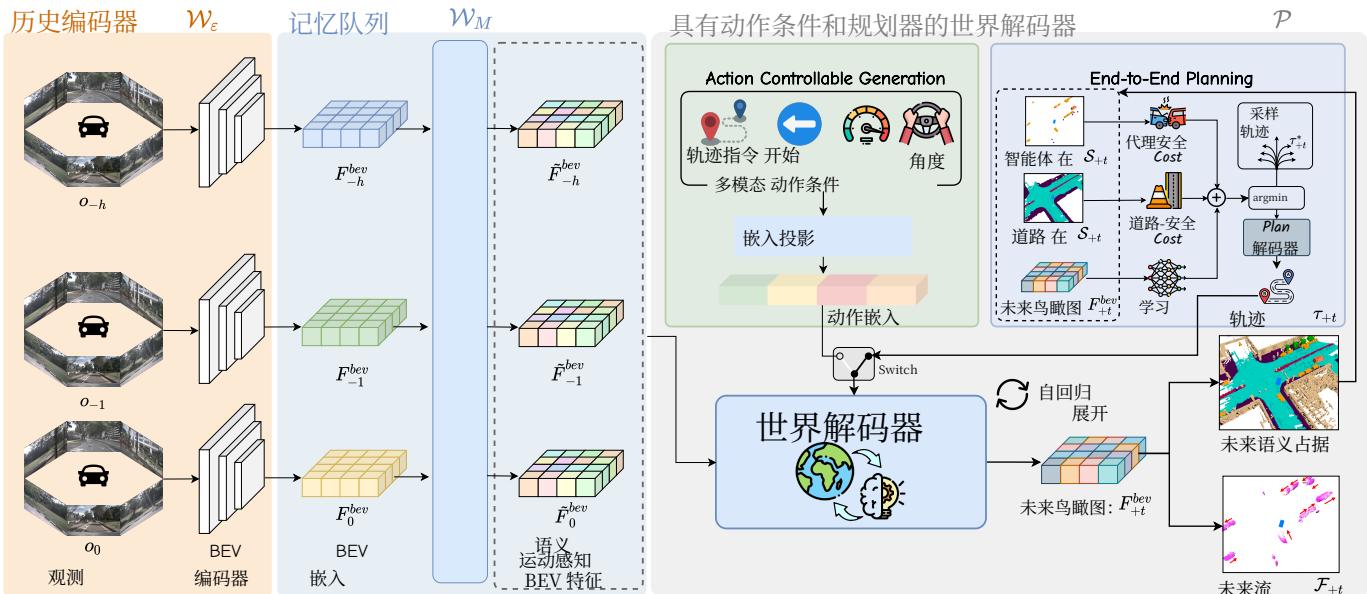
图 2：Drive‑OccWorld 概览。（a）历史编码器提取多视角图像特征并将其转换为 BEV 嵌入。（b）记忆队列使用语义与运动条件归一化来聚合历史信息。（c）世界解码器结合动作条件以生成多种未来占用和流场。将世界解码器与基于占据的规划器结合，可实现连续预测与规划。

在本工作中，我们通过注入动作条件来探索世界模型的潜在应用，以实现可由动作控制的生成，并将这种生成能力与端到端规划器集成以实现安全驾驶。

3 方法

3.1 预备知识

端到端自动驾驶模型旨在基于传感器输入和自车动作（即，规划轨迹）直接控制车辆（ $\mathrm{Hu}$ 等人 2023b）。形式上，给定在 $h$ 个时间戳上的历史传感器观测 {o−h,…,o−1,o0}\{ o _ { - h } , \ldots , o _ { - 1 } , o _ { 0 } \}{o−h​,…,o−1​,o0​} 和自车轨迹 {τ−h,…,τ−1,τ0}\{ \tau _ { - h } , \ldots , \tau _ { - 1 } , \tau _ { 0 } \}{τ−h​,…,τ−1​,τ0​} ，端到端模型 $\mathcal{A}$ 预测未来 $f$ 个时间戳的期望自车轨迹 {τ1,…,τf}\{ \tau _ { 1 } , \ldots , \tau _ { f } \}{τ1​,…,τf​} ：

A({o−h,…,o−1,o0},{τ−h,…,τ−1,τ0})={τ1,…,τf} A ( \{ o _ { - h } , \ldots , o _ { - 1 } , o _ { 0 } \} , \{ \tau _ { - h } , \ldots , \tau _ { - 1 } , \tau _ { 0 } \} ) = \{ \tau _ { 1 } , \ldots , \tau _ { f } \} A({o−h​,…,o−1​,o0​},{τ−h​,…,τ−1​,τ0​})={τ1​,…,τf​}

驾驶世界模型 $\mathcal{W}$ 可以被看作一种生成模型，它以先前的观测和自车动作 {a−h,…,a−1,a0}\{ a _ { - h } , \dotsc , a _ { - 1 } , a _ { 0 } \}{a−h​,…,a−1​,a0​} 为输入，生成环境的合理未来状态 {s1,…,sf}\{ s _ { 1 } , \ldots , s _ { f } \}{s1​,…,sf​} ：W({o−h,…,o−1,o0},{a−h,…,a−1,a0})={s1,…,sf}{ \mathcal { W } } ( \{ o _ { - h } , \ldots , o _ { - 1 } , o _ { 0 } \} , \{ a _ { - h } , \ldots , a _ { - 1 } , a _ { 0 } \} ) = \{ s _ { 1 } , \ldots , s _ { f } \}W({o−h​,…,o−1​,o0​},{a−h​,…,a−1​,a0​})={s1​,…,sf​} (2)其中自车动作 $a$ 可以以各种形式注入到可控生成过程中，即 速度、转向角、自车轨迹以及高层指令。

鉴于 world model 预测未来状态的能力，我们提出将其与规划器集成以充分利用

world model 在端到端规划中的能力。具体而言，我们引入了一个称为 Drive‑OccWorld 的自回归框架，该框架由一个生成式 world model $\mathcal{W}$ 组成，用于预测未来的占用和流状态，以及一个基于占据的规划器 $\mathcal{P}$ ，该规划器使用代价函数通过评估未来预测来选择最优轨迹。形式上，我们将 Drive‑OccWorld 表述如下，该模型自回归地预测下一个时间戳的未来状态和轨迹：

W({o−h,…,o−1,o0},{s1,…,st−1,st},{a−h,…,a−1,a0,…,at−1,at} ds)=st+1 \begin{array} { c } { { { \mathcal { W } ( \{ o _ { - h } , \dotsc , o _ { - 1 } , o _ { 0 } \} , \{ s _ { 1 } , \dotsc , s _ { t - 1 } , s _ { t } \} , } } } \\ { { { \{ a _ { - h } , \dotsc , a _ { - 1 } , a _ { 0 } , \dotsc , a _ { t - 1 } , a _ { t } \} \ d s ) = s _ { t + 1 } } } } \end{array} W({o−h​,…,o−1​,o0​},{s1​,…,st−1​,st​},{a−h​,…,a−1​,a0​,…,at−1​,at​} ds)=st+1​​

$$\mathcal{P}(f_o(s_{t+1},{\tau }_{t+1}^{\ast }))={\tau }_{t+1}$$

其中 $f_o$ 是基于占用的代价函数， ${\tau }_{t+1}^{\ast }$ 表示在时间戳 $t+1$ 处采样的轨迹候选。

值得注意的是，对于可控动作生成， $a$ 可以作为速度等形式的条件注入到 $\mathcal{W}$ 中，等，并且为了防止潜在的自车状态泄露，会丢弃 $\mathcal{P}$ 。在端到端规划中，预测轨迹 ${\tau }_{t+1}$ 作为动作条件$a_{t+1}$ 用于预测下一个状态 $s_{t+2}$ ，从而导致预测与规划的连续展开。

在下列部分中，我们将详细说明世界模型的结构，使 $\mathcal{W}$ 具备可控动作生成能力，并将其与 $\mathcal{P}$ 集成以实现端到端规划。

3.2 使用世界模型的4D 预测

如图2所示，Drive‑OccWorld 包含三个组件：(1) 一个 历史编码器 ${\mathcal{W}}_{\mathcal{E}}$ ，该编码器以历史摄像头图像为输入，提取多视图几何特征，并将其转换为 BEV 嵌入。继承先前工作（Yang et al. 2024b；Min et al. 2024），我们采用视觉BEV 编码器（Li et al. 2022）作为我们的历史编码器。(2)一个 记忆队列 $w_{\mathcal{M}}$ 与语义-

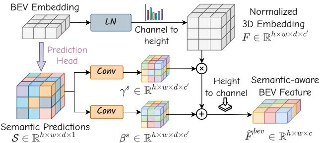
Figure 3: Overview of semantic-conditional normalization.

and Motion-Conditional Normalization, which employs a simple yet efficient normalization operation in latent space to aggregate semantic information and compensate for dynamic motions, thereby accumulating more representative BEV features. (3) a World Decoder ${\mathcal{W}}_{\mathcal{D}}$ , which extracts world knowledge through temporal modeling with historical features to forecast future semantic occupancies and flows. Flexible action conditions can be injected into ${\mathcal{W}}_{\mathcal{D}}$ for controllable generation. An occupancy-based planner $\mathcal{P}$ is integrated for continuous forecasting and planning.

Semantic- and Motion-Conditional Normalization is designed to enhance historical BEV embeddings by incorporating semantic and dynamic information. For example, consider the BEV embedding $F^{bev}\in {\mathbb{R}}^{h\times w\times c}$ , where $h$ and $w$ are the spatial resolutions of the BEV, and $c$ denotes the channel dimension. We first apply layer normalization without affine mapping, then modulate it into ${\tilde{F}}^{bev}$ using an adaptive affine transformation, with the scale and shift parameters $({\gamma }^{\ast },{\beta }^{\ast })$ derived from semantic or motion labels:

$${\tilde{F}}^{bev}={\gamma }^{\ast }\cdot LayerNorm(F^{bev})+{\beta }^{\ast }$$

Specifically, for semantic-conditional normalization, $({\gamma }^s,{\beta }^s)$ are inferred from voxel-wise semantic predictions. As illustrated in Figure 3, we implement a lightweight head along with the argmax function to predict voxel-wise semantic labels $\mathcal{S}\in {\breve{\mathbb{R}}}^{h\times w\times d\times 1}$ , where $d$ denotes the height of the voxelized 3D space. The semantic labels are encoded as one-hot embeddings and convolved to produce modulation parameters for the affine transformation as Eq. 5. This method efficiently enhances the semantic discrimination of BEV embeddings, as demonstrated in the experiments.

In motion-conditional normalization, we account for the movements of both the ego vehicle and other agents across various timestamps. Specifically, the ego-pose transformation matrix KaTeX parse error: Undefined control sequence: \ot at position 32: …+ t } \doteq [ \̲o̲t̲ ̲{ R } _ { - t }… , which represents the rotation and translation of the ego vehicle from timestamp $-t$ to $+t$ , is flattened and encoded into an embedding processed by MLPs to generate affine transformation parameters $({\gamma }^e,{\beta }^e)$ . To address the movements of other agents, we predict voxelwise 3D backward centripetal flow $\mathcal{F}\in {\mathbb{R}}^{\hat{h}\times w\times d\times 3}$ that points from the voxel at time $t$ to its corresponding 3D instance center at $t-1$ , and encode it into $(\grave{{\gamma }^f},{\beta }^f)$ for finegrained motion-aware normalization using Eq. 5.

Future Forecasting with World Decoder. ${\mathcal{W}}_{\mathcal{D}}$ is an autoregressive transformer that predicts the BEV embeddings $F_{+t}^{\overline{b}ev}$ for the future frame $+t$ based on historical BEV features stored in $w_{\mathcal{M}}$ and the expected action condition $a_{+t}$ .

Specifically, ${\mathcal{W}}_{\mathcal{D}}$ takes learnable BEV queries as input and performs deformable self-attention, temporal crossattention with historical embeddings, conditional crossattention with action conditions, and a feedforward network to generate future BEV embeddings. The conditional layer performs cross-attention between BEV queries and action embeddings, which will be illustrated in the following section, injecting action-controllable information into the forecasting process. After obtaining the next BEV embeddings F bev, prediction heads utilizing the channel-to-height operation (Yu et al. 2023) to predict semantic occupancy and 3D backward centripetal flow (S+t, F+t) ∈ Rh×w×d.

In the training process, we employ multiple losses, including cross-entropy loss, Lovasz loss ( ´ Berman, Rannen Triki, and Blaschko 2018), and binary occupancy loss, to constrain the semantics and geometries of occupancy predictions $ { \mathcal { S } } _ { 1 : f }$ . The $l_1$ loss is used to supervise flow predictions ${\mathcal{F}}_{1:f}$ .

3.3 Action-Controllable Generation

Due to the inherent complexity of the real world, the motion states of the ego vehicle are crucial for the world model to understand how the agent interacts with its environment. Therefore, to fully comprehend the environment, we propose leveraging diverse action conditions to empower DriveOccWorld with the capability for controllable generation.

Diverse Action Conditions include multiple formats: (1) Velocity is defined at a given time step as $(v_x,v_y)$ , representing the speeds of the ego vehicle decomposed along the $x$ and $y$ axes in $m/s$ . (2) Steering Angle is collected from the steering feedback sensor. Following VAD, we convert it into curvature in $m^{-1}$ , indicating the reciprocal of the turning radius while considering the geometric structure of the ego car. (3) Trajectory represents the movement of the ego vehicle’s location to the next timestamp, formulated as $(△x,△y)$ in meters. It is widely used as the output of endto-end methods, including our planner $\mathcal{P}$ . (4) Commands consist of go forward, turn left, and turn right, which represent the highest-level intentions for controlling the vehicle.

Unified Conditioning Interface is designed to incorporate heterogeneous action conditions into a coherent embedding, inspired by (Gao et al. 2024; Wang et al. 2024b). We first encode the required actions via Fourier embeddings (Tancik et al. 2020), which are then concatenated and fused via learned projections to align with the dimensions of the conditional cross-attention layers in ${\mathcal{W}}_{\mathcal{D}}$ . This method enables efficient integration of flexible action conditions into controllable generation, with experiments demonstrating that the unified interface with conditional crossattention provides superior controllability compared to other approaches such as additive embeddings.

3.4 End-to-End Planning with World Model

Existing world models primarily focus on either data generation or the pertaining paradigms for autonomous driving. Although a recent pioneering work, Drive-WM (Wang et al. 2024b), proposed integrating generated driving videos with an image-based reward function to plan trajectories, 和运动条件归一化，该方法在潜在空间中采用一种简 单但高效的归一化操作来聚合语义信息并补偿动态运 动，从而累积更具代表性的 BEV 特征。(3) 一个 世界 解码器 ${\mathcal{W}}_{\mathcal{D}}$ ，通过对历史特征进行时序建模来提取世 界知识，以预测未来语义占据和流场。可将灵活的动 作条件注入到 ${\mathcal{W}}_{\mathcal{D}}$ 以实现可控生成。一个基于占据的 规划器 $\mathcal{P}$ 被集成用于连续预测与规划。

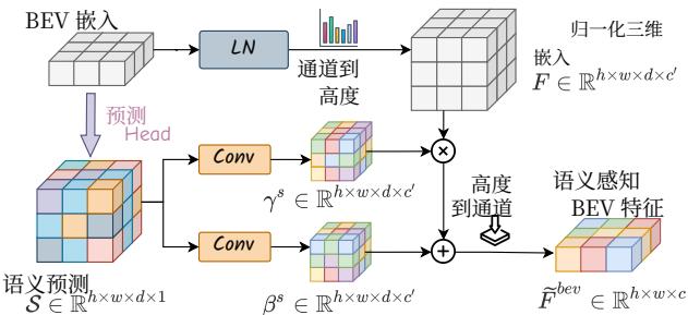
图 3：语义条件归一化概览。

Semantic-and Motion-Conditional Normalization 旨在通过融合语义和动态信息来增强历史 BEV 嵌入。例如，考虑 BEV 嵌入 $F^{bev}\in {\mathbb{R}}^{h\times w\times c}$ ，其中 $h$ 和 $w$ 是 BEV 的空间分辨率， $c$ 表示通道维度。我们首先应用不带仿射映射的层归一化，然后通过自适应仿射变换将其调制为 ${\tilde{F}}^{bev}$ ，缩放和平移参数 $({\gamma }^{\ast },{\beta }^{\ast })$ 来自语义或运动标签：

$${\tilde{F}}^{bev}={\gamma }^{\ast }\cdot LayerNorm(F^{bev})+{\beta }^{\ast }$$

具体来说，对于语义条件归一化， $({\gamma }^s,{\beta }^s)$ 由体素级语义预测推断。正如图3所示，我们实现了一个轻量级头并结合argmax函数来预测体素级语义标签$S\in {\mathbb{R}}^{h\times w\times d\times 1}$ ，其中 $d$ 表示体素化三维空间的高度。语义标签以独热嵌入编码并经过卷积以产生用于仿射变换的调制参数，如等式5所示。实验表明，该方法有效增强了BEV嵌入的语义判别能力。

在运动条件归一化中，我们考虑了自车和其他智能体在不同时间戳上的运动。具体来说，表示自车从时间戳 $-t$ 到 $+t<$ <style id $\lfloor {=}^{\prime }10^{\prime }\}$ 旋转和平移的自车位姿变换矩阵 $E_{-t}^{+t}=[R_{-t}^{+t},T_{-t}^{+t}].$ ，被展平并编码为一个嵌入，通过多层感知机处理以生成仿射变换参数 $({\gamma }^e,{\beta }^e{)}_{\circ }$ 。为了解决其他智能体的运动，我们预测指向从时间 $t$ 的体素到其对应在 $t-1$ 处的三维实例中心的体素级三维反向向心流 $\mathcal{F}\in {\mathbb{R}}^{h\times w\times d\times 3}$ ，并将其编码为 $({\gamma }^f,{\beta }^f)$ ，用于基于等式5的细粒度运动感知归一化。

Future Forecasting with WorldDecoder. ${\mathcal{W}}_{\mathcal{D}}$ 是一个自回归变换器，根据存储在 $w_{\mathcal{M}}$ 中的历史BEV特征和期望的动作条件 $a_{+t}$ ，预测未来帧 $+t$ 的BEV嵌入 $F_{+t}^{bev}{}_{}$ 。

具体来说， ${\mathcal{W}}_{\mathcal{D}}$ 以可学习的BEV查询作为输入，执行可变形自注意力、与历史嵌入的时序交叉注意力、与动作条件的条件交叉注意力，以及一个前馈网络以生成未来BEV嵌入。条件层在BEV查询和动作嵌入之间执行交叉注意力（将在下节中说明），将可由动作控制的信息注入预测过程。在获得下一个BEV嵌入 $F_{+t}^{bev}$ 后，预测头利用通道到高度的操作（Yu et al. 2023）来预测语义占据和三维反向向心流 $(S_{+t},{\mathcal{F}}_{+t})\in {\mathbb{R}}^{h\times w\times d}\mathrm{c}$ 。

在训练过程中，我们使用多种损失，包括交叉熵损失、Lov´asz 损失（Berman、Rannen Triki 和Blaschko 2018）以及二值占用损失，以约束占据预测的语义和几何形状 ${\mathcal{S}}_{1:f\circ }$ 。 $l_1$ 损失用于监督流预测 ${\mathcal{F}}_{1:f\circ }$

3.3 可控动作生成

由于现实世界的固有复杂性，自车的运动状态对于世界模型理解智能体如何与环境交互至关重要。因此，为了充分理解环境，我们提出利用多样的动作条件来赋能 Drive‑OccWorld，使其具备可控生成的能力。

多样动作条件 包含多种形式：(1)速度 在给定时间步定义为 $(v_x,v_y)$ ，表示将自车的速度沿 $x$ 和 $y$ 轴在 $m/s$ 中分解的分量。(2) 转向角 由转向反馈传感器采集。参照 VAD，我们将其转换为 $m^{-1}$ 中的曲率，表示考虑自车几何结构后的转弯半径的倒数。(3) 轨迹 表示自车位置到下一时间戳的移动，形式化为以米为单位的$(△x,△y)$ 。它作为端到端方法（包括我们的规划器 $\mathcal{P}$ ）的输出被广泛使用。(4) 指令由前进、向左转和向右转组成，代表用于控制车辆的最高级别意图。

UnifiedConditioningInterface 旨在将异构的动作条件融入为一致的嵌入，灵感来自 (Gao 等人 2024；Wang 等人 2024b)。我们首先通过傅里叶嵌入（Tancik 等人 2020）对所需动作进行编码，然后将这些编码串联并通过学习到的投影融合，以对齐 ${\mathcal{W}}_{\mathcal{D}}$ 中条件交叉注意力层的维度。该方法使灵活的动作条件能够高效地集成到可控生成中，实验证明，与加性嵌入等其他方法相比，结合条件交叉注意力的统一接口提供了更优越的可控性。

3.4 使用 WorldModel 的端到端规划

现有的世界模型主要侧重于数据生成或与自动驾驶相关的范式。尽管最近一项开创性工作 Drive‑WM(Wang 等人 2024b) 提出将生成的驾驶视频与基于图像的奖励函数相结合以用于规划轨迹，

the geometric 3D features of the environment are not fully exploited for motion planning. Leveraging the future occupancy forecasting capabilities of our world model, as illustrated in Figure 2, we introduce an occupancy-based planner that samples occupied grids of agents and drivable areas to enforce safety constraints. Additionally, we employ a learned-volume cost to provide a more comprehensive evaluation of the environment for safe planning.

Occupancy-based Cost Function is designed to ensure the safe driving of the ego vehicle. It consists of multiple cost factors: (1) Agent-Safety Cost constrains the ego vehicle from colliding with other agents, such as pedestrians and vehicles. It penalizes trajectory candidates that overlap with grids occupied by other road users. Additionally, trajectories that are too close to other agents, in terms of lateral or longitudinal distance, are also restricted to avoid potential collisions. (2) Road-Safety Cost ensures the vehicle remains on the road. It extracts road layouts from occupancy predictions, penalizing trajectories that fall outside the drivable area. (3) Learned-Volume Cost is inspired by ST-P3 (Hu et al. 2022). It employs a learnable head based on $F_{+t}^{bev}$ to generate a 2D cost map, enabling a more comprehensive evaluation of occupancy grids in complex environments.

The total cost function is the summation of the above cost factors. Following the approach of ST-P3, a trajectory sampler generates a set of candidate trajectories ${\tau }_{+t}^{\ast }\in {\dot{\mathbb{R}}}^{N_{\tau }\times 2}$ distributed across the 2D grid map surrounding the ego vehicle, guided by high-level commands. Subsequently, the trajectory planner $\mathcal{P}$ selects the optimal trajectory ${\tau }_{+t}$ by minimizing the total cost function, while simultaneously ensuring agent and road safety.

BEV Refijectory usi ent is introduced to further refine thhe latent features of BEV embeddings $F_{+t}^{bev}$ ${\tau }_{+t}$ command embedding to form an ego query, which performs cross-attention with ${\bar{\mathbf{\Pi }}}_{F_{+t}^{bev}}$ to extract fine-grained representations of the environment. The final trajectory is predicted based on the refined ego query through MLPs.

The planning loss ${\mathcal{L}}_{plan}$ consists of three components: a max-margin loss introduced by (Sadat et al. 2020) to constrain the safety of trajectory candidates ${\tau }_{+t}^{\ast }$ , a naive $l_2$ loss for imitation learning, and a collision loss that ensures the planned trajectory avoids grids occupied by obstacles. Notably, when performing end-to-end planning, we utilize the predicted trajectories as action conditions for both training and testing. This approach not only prevents GT ego actions from leaking into the planner but also facilitates model learning using predicted trajectories, enabling improved performance during testing.

4 Experiments

4.1 Setup

We conduct experiments on the nuScenes (Caesar et al. 2020), nuScenes-Occupancy (Wang et al. 2023c), and LyftLevel5 datasets. More details regarding the experimental implementation are provided in the appendix.

Tasks Definition. We validate Drive-OccWorld’s effectiveness in 4D occupancy and flow forecasting, which includes inflated and fine-grained occupancy formats, as well as trajectory planning. (1) Inflated GMO and Flow Forecasting is presented in Cam4DOcc (Ma et al. 2024b), predicting the future states of general movable objects (GMO) with dilated occupancy patterns. The dataset is constructed by transforming movable objects at different timestamps into the present coordinate system, voxelizing the 3D space, and labeling grids with semantic and instance annotations. Voxel grids within bounding boxes are marked as GMO, and the 3D backward centripetal flow indicates the direction of voxels in the current frame toward their corresponding 3D instance centers from the previous timestamp. (2) Fine-Grained GMO Forecasting predicts occupied grids of GMO using voxel-wise labels from the nuScenes-Occupancy dataset. (3) Fine-grained GMO and GSO Forecasting predicts the voxel-wise labels for both general movable objects (GMO) and general static objects (GSO) based on fine-grained annotations from nuScenesOccupancy. (4) End-to-end Planning follows the open-loop evaluation on nuScenes.

Metrics. (1) Occupancy forecasting is evaluated using the mIoU metric. Following Cam4DOcc, we assess the current moment $(t=0$ ) with ${\mathrm{mIoU}}_c$ and the future timestamps $(t\in [1,f])$ with ${\mathrm{mIoU}}_f$ . Additionally, we provide a quantitative indicator ${\widetilde{\mathrm{mIoU}}}_f$ weighted by timestamp, in line with the principle that occupancy predictions at nearby timestamps are more critical for planning. (2) Flow predictions are evaluated through instance association using the video panoptic quality ${\mathrm{VPQ}}_f$ metric. We further report the flow forecasting results denoted as ${\mathrm{VPQ}}_f^{\ast }$ , utilizing a simple yet efficient center clustering technique, where the predicted object centers are clustered based on their relative distances. (3) End-to-end planning is evaluated using the L2 distance from ground truth trajectories and the object collision rate. More details of the metrics are provided in the appendix.

4.2 Main Results of 4D Occupancy Forecasting

First, we verify the quality of 4D occupancy forecasting and the controllable generation capabilities of Drive-OccWorld. We report performance conditioned on ground-truth actions as Drive- $\dot{{\mathrm{OccWorld}}^A}$ , and results conditioned on predicted trajectories from the planner $\mathcal{P}$ as Drive-OccWorldP .

Inflated GMO and Flow Forecasting. Table 1 presents comparisons of inflated GMO and flow forecasting on the nuScenes and Lyft-Level5 datasets. Drive-OccWorld outperforms previous methods on various time intervals, including the performance on the current moment and future timestamps. For instance, it surpasses Cam4DOcc on the ${\widetilde{\mathrm{mIoU}}}_f$ metric by $9.4\%$ and $6\%$ on nuScenes and Lyft-Level5, respectively. The results demonstrate Drive-OccWorld’s superior ability to forecast future world states.

For future flow predictions, Drive-OccWorldP outperforms previous SoTA methods by $5.1\%$ and $5.2\%$ on ${\mathrm{VPQ}}_f$ for nuScenes and Lyft-Level5, respectively, indicating superior capability in modeling dynamic object motions.

然而，环境的几何三维特征在运动规划中尚未被充分利用。正如图2所示，我们利用世界模型的未来占用预测能力，引入了一种基于占用的规划器，通过对智能体和可行驶区域的占用网格进行采样来强制执行安全约束。此外，我们还采用了一种学习体积代价，以便对安全规划的环境提供更全面的评估。

基于占用的代价函数 旨在确保自车的安全驾驶。它由多个代价因子组成：(1) 代理安全代价 约束自车避免与其他智能体（如行人和车辆）发生碰撞。它会惩罚与被其他道路使用者占据的格子重叠的轨迹候选。此外，从横向或纵向距离上与其他智能体过于接近的轨迹也会被限制，以避免潜在的碰撞。(2) 道路安全代价 确保车辆保持在道路上。它从占据预测中提取道路布局，惩罚落在可行驶区域之外的轨迹。(3) 学习体积代价 的灵感来自 ST‑P3（Hu 等人 2022）。它基于 $F_{+t}^{bev}$ 使用可学习的 head 来生成二维代价图，从而在复杂环境中对占用网格进行更全面的评估。

总代价函数是上述各代价因子的总和。沿用ST‑P3 的方法，轨迹y 采样器生成一组轨迹候选${\tau }_{+t}^{\ast }\in {\mathbb{R}}^{N_{\tau }\times 2}$ ，这些候选沿围绕自车的二维网格地图分布，并由高层指令引导。随后，轨迹规划器 $\mathcal{P}$ 通过最小化总代价函数来选择最优轨迹 ${\tau }_{+t}$ ，同时确保代理和道路的安全性。

鸟瞰视图（BEV）精化被引入以利用 BEV 嵌入的潜在特征 $F_{+t}^{bev}$ 进一步精化轨迹。我们将 ${\tau }_{+t}$ 编码成一个嵌入，并将其与指令嵌入串联以形成自车查询，该查询对 $F_{+t}^{bev}$ 执行交叉注意力以提取环境的细粒度表示。最终轨迹基于通过多层感知机（MLPs）精化后的自车查询进行预测。

规划损失 ${\mathcal{L}}_{plan}$ 由三部分组成：由 Sadat 等人2020 引入的最大间隔损失，用以约束轨迹候选的安全性 ${\tau }_{+t}^{\ast }$ ；用于模仿学习的简单 $l_2$ 损失；以及确保规划轨迹避开被障碍物占据网格的碰撞损失。值得注意的是，在执行端到端规划时，我们使用预测轨迹作为训练和测试的动作条件。这种方法不仅防止了 GT 自车动作泄露到规划器中，而且通过使用预测轨迹来辅助模型学习，使测试阶段性能得以提升。

4 实验

4.1 设置

我们在 nuScenes (Caesar 等人 2020)、nuScenes‑Occupancy (Wang 等人 2023c) 和 Lyft‑Level5 数据集上进行了实验。关于实验实现的更多细节见附录。

Tasks Definition. 我们验证 Drive‑OccWorld 在 4D 占据 和 流量预测 方面的有效性，包含膨胀和细粒度占据格式，以及轨迹规划。 (1) Inflated GMO and FlowForecasting 在 Cam4DOcc (Ma et al. 2024b) 中给出，预测具有膨胀占据模式的general movableobjects (GMO)的未来状态。该数据集通过将不同时间戳的可移动物体变换到当前坐标系、对 3D 空间进行体素化，并使用语义和实例标注为网格打标签来构建。位于边界框内的体素网格被标记为 GMO，三维反向向心流 指示当前帧中的体素朝向其在先前时间戳对应的 3D 实例中心的方向。 (2)

Fine-Grained GMO Forecasting使用来自
nuScenes‑Occupancy 数据集的逐体素标签预测 GMO 的被占据网格。(3) Fine-grained GMO andGSOForecasting 基于 nuScenes‑Occupancy 的细粒度标注，预测general movable objects (GMO)和general static
objects(GSO)的逐体素标签。 (4) End-to-end Planning 在nuScenes 上遵循开环评估。

评估指标。 (1) 占用预测使用 mIoU 指标进行评估。遵循 Cam4DOcc，我们评估当前时刻 $(t=0$ ) 的${\mathrm{mIoU}}_c$ ，以及未来时间戳（ $\left(t\in \left[1,f\right]\right)$ ）的 $\mathrm{mIoU}f$ 。此外，我们还提供按时间戳加权的定量指标 $\mathrm{mIoU}f$ ，基于占用预测在相近时间戳对规划更为关键的原则。(2)流预测通过使用视频全景质量 $\mathrm{VPQ}f$ 的实例关联来评估。我们还报告记为 ${\mathrm{VPQ}}_f^{\ast }$ 的流预测结果，采用一种简单但高效的中心聚类技术，将预测的对象中心按相对距离进行聚类。(3) 端到端规划 使用与真实轨迹的 L2 距离和物体碰撞率进行评估。更多评估指标细节见附录。

4.2 4D 占据预测的主要结果

首先，我们验证了 Drive‑OccWorld 在 4D 占用预测以及可控生成 能力的质量。我们报告了以真实动作为条件的性能，记为 Drive‑OccWorldA，以及以规划器预测轨迹为条件的结果 $\mathcal{P}$ ，记为 Drive‑OccWorldP。膨胀可移动物体和流预测。表1 给出了在 nuScenes 和Lyft‑Level5 数据集上膨胀可移动物体和流预测的比较。Drive‑OccWorld 在多个时间间隔上优于以往方法，包括当前时刻和未来时刻的表现˜。例如，它在 mIoUf指标上分别比 Cam4DOcc 在 nuScenes 和 Lyft‑Level5 上高出 $9.4\%$ 和 $6\%$ 。这些结果证明了 Drive‑OccWorld 在预测未来世界状态方面的优越能力。

对于未来流预测，Drive‑OccWorldP 在VPQf 上分别比之前的最优方法在nuScenes和Lyft‑Level5上高出 $5.1\%$ 和$5.2\%$ ，表明其在建模动态物体运动方面具有更强的能力。

Method	Inflated GMO								Fine-Grained GMO
	nuScenes				Lyft-Level5				nuScenes-Occupancy mIoUc mloUf (2 s) mloUf
	mIoUc mIoUf (2 s) mIoUf VPQf|IoUc mIoUf (0.8 s) mIoUf VPQf|
SPC	1.3	failed	failed	1	1.4	failed	failed	/	5.9	1.1	1.1
OpenOccupancy-C (Wang et al. 2023c)	12.2	11.5	11.7		14.0	13.5	13.7		10.8	8.0	8.5
PowerBEV-3D (Li et al. 2023a)	23.1	21.3	21.9	20.0	26.2	24.5	25.1 34.6	27.4	5.9	5.3	5.5
Cam4DOcc (Ma et al. 2024b)	31.3	26.8	28.0	18.6	36.4	33.6		28.2	11.5	9.7	10.1
Drive-OccWorld4 (Ours)	39.7	36.3	37.3	23.7	40.6	39.3	40.0	32.2	13.6	11.9	12.3
Drive-OccWorldP (Ours)	39.8	36.3	37.4	25.1	40.9	39.7	40.6	33.4	13.6	12.0	12.4

SPC: SurroundDepth (Wei et al. 2023a) ${}^{+}$ PCPNet (Luo et al. 2023) ${}^{+}$ Cylinder3D (Zhu et al. 2021)

Table 1: Comparisons of Inflated GMO and Flow Forecasting on the nuScenes and Lyft-Level5 datasets, and Fine-Grained GMO Forecasting on the nuScenes-Occupancy dataset, with the top two results highlighted in bold and underlined text.

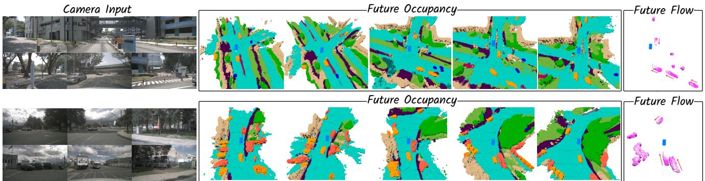
Figure 4: Qualitative results of 4D occupancy and flow forecasting. The results are presented at various future timestamps.
Table 3: Comparisons of controllability under diverse action conditions, with the top two results highlighted in bold and underlined. ${✓}^{\mathcal{P}}$ denotes the predicted trajectory.

Table 2: Comparisons of Fine-Grained GMO and GSO Forecasting on nuScenes-Occupancy dataset.

Method	mIoUc mIoUf(2s）mloUf
	5 00 8mean meanGMO
SPCPowerBEV-3D (Li et al.2023a)CONet-C (Wang et al.2023c)Cam4DOcc (Ma et al. 2024b)	5.93.34.61.11.41.2 1.15.91 15.31 1 5.59.6 17.2 13.4 7.4 17.3 12.47.911.0 17.8 14.4 9.2 17.8 13.59.7
DriveOccWorldA (Ours)DriveOccWorldP (Ours)	16.6 20.2 18.4 14.3 21.4 17.8 14.916.9 20.2 18.5 14.3 21.2 17.8 14.9

SPC: SurroundDepth (Wei et al. 2023a) ${}^{+}$ PCPNet (Luo et al. 2023) ${}^{+}$ Cylinder3D (Zhu et al. 2021)

Fine-Grained GMO Forecasting. Fine-grained GMO forecasting poses more challenges than inflated GMO forecasting, since it requires predicting more fine-grained voxel labels than the bounding-box level labels. Table 1 presents comparisons of fine-grained GMO forecasting on the nuScenes-Occupancy dataset. The results show that Drive-OccWorld still outperforms previous methods across all time intervals, showcasing Drive-OccWorld’s ability to forecast more fine-grained world states.

Fine-grained GMO and GSO Forecasting. Table 2 presents comparisons of fine-grained GMO and GSO forecasting on the nuScenes-Occupancy dataset. The results demonstrate that Drive-OccWorld achieves the best performance among all approaches. Notably, Drive-OccWorldP outperforms Cam4DOcc by $5.9\%$ and $5.1\%$ on mIoU for general movable objects (GMO) at current and future timestamps, respectively, illustrating its ability to accurately locate movable objects for safe navigation. Figure 4 provides qualitative results of fine-grained occupancy forecasting and flow predictions across frames.

No.	Action Condition traj vel angle cmd		mIoUcmIoUf(1s) mloUf 28.7	26.4	26.8	VPQ 33.5
1 4	√ √	√ √	28.5 28.9个0.2 28.9个0.2 29.2个0.5	27.6个1.2 27.5个1.1 26.8个0.4 26.8个0.4	27.8个1.0 27.8个1.0 27.2个0.4 27.3个0.5	33.7个0.2 33.9个0.4 34.2+0.7 34.7个1.2
5 6 7P	√ ▼	√ 一	29.0个0.3 29.2 ↑0.5	27.6个1.2 27.9 个1.5	27.8个1.0 28.1个1.3	35.0个1.5 35.1个1.6

Controllability. Table 3 examines controllability under various action conditions. Injecting any action condition improves results compared to the baseline. Low-level conditions, such as trajectory and velocity, significantly enhance future forecasting $(\mathrm{m}\widetilde{\mathrm{Io}}{\mathrm{U}}_f)$ ), while high-level conditions, such as commands, boost results at the current moment ${(\mathrm{mIoU}}_c)$ ) but have limited impact on future predictions. We explain that incorporating more low-level conditions helps the world model better understand how the ego vehicle interacts with the environment, thereby improving forecasting performance.

方法	Inflated GMO								细粒度GMO
	nuScenes										nuScenes-Occupancy
	mIoUcmIoUf(2秒) mIoUfVPQfIUcmIoUf(0.8秒) mIoUfVPQfmIbUmIoUf(2秒) mIoUf
SPC	1.3		购	1	1.4				/	5.9	1.1		1.1
OpenOccupancy-C (Wang et al. 2023c)1	12.2					14.0			1	10.8		8.0	8.5
PowerBEV-3D (Li et al.2023a)	23.1	21.3		21.9	20.026.2		24.5	25.1	27.4	5.9		5.3	5.5
Cam4DOcc (Ma et al. 2024b)	31.3	26.8		28.0	18.636.4		33.6	34.6	28.2	11.5		9.7	10.1
Drive-OccWorld4(我们的（Ours））	39.7	36.3		37.3	23.74		39.3	40.0	32.2	13.6		11.9	12.3
Drive-OccWorldP(我们的（Ours））	39.8	36.3		37.4	25.14		39.7	40.6	33.4		13.6	12.0	12.4

SPC: SurroundDepth (Wei 等，2023a) $\overline{+}$ PCPNet (Luo 等，2023) $\overline{+}$ Cylinder3D (Zhu 等，2021)

表 1：在 nuScenes 和 Lyft‑Level5 数据集上比较膨胀可移动物体和流预测，以及在 nuScenes‑Occupancy 数据集上比较细粒度GMO预测，前两名结果以加粗并带下划线的文本标注。

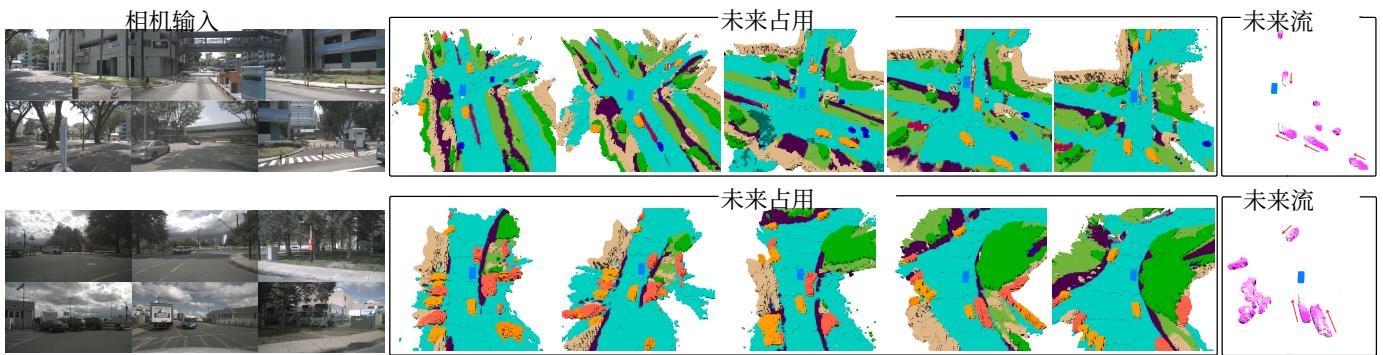
图 4：4D 占据和流量预测的定性结果。结果在不同的未来时间戳下展示。

方法	mIoUc mIoUf (2 s)	mIoUf A
SPC 5.9 3.3 4.6 1.1 PowerBEV-3D(Lietal.2023a) 5.9--5.3-- CONet-C (Wang etal. 2023c)9.6 17.213.47.417.3 12.4 Cam4DOcc(Maet al. 2024b) 11.017.8 14.49.217.8 13.5	1.41.2	1.1 5.5 7.9
DriveOccWorldA(我们的（Ours）） DriveOccWorldP(我们的（Ours）)	16.6 16.9	9.7 14.9 14.9

SPC: SurroundDepth (Wei 等，2023a) +PCPNet (Luo 等，2023) ${}^{+}$ Cylinder3D (Zhu 等，2021)

表2：在 nuScenes‑Occupancy 数据集上比较细粒度GMO 与 GSO 预测。

细粒度 GMO 预测。细粒度 GMO 预测比膨胀型GMO 预测更具挑战性，因为它需要预测比边界框级别标签更为细化的体素标签。表1给出了在nuScenes‑Occupancy 数据集上细粒度 GMO 预测的比较。结果显示，Drive‑OccWorld 在所有时间间隔上仍然优于之前的方法，展示了 Drive‑OccWorld 预测更细粒度世界状态的能力。

细粒度 GMO 与 GSO 预测。 表 2展示了在nuScenes‑Occupancy 数据集上细粒度 GMO 与 GSO预测的比较。结果表明 Drive‑OccWorld 在所有方法中表现最佳。值得注意的是，Drive‑OccWorldP在mIoU 上分别比 Cam4DOcc 提高了 $5.9\%$ 和 $5.1\%$

No.	动作条件 轨迹 速度 角度控制命令	mIoUc		"mIoUf (1秒)mIoUf		VPQ
1 2	√		28.7 28.5		26.4 27.6个1.2	26.8	33.5 33.710.2
3	√	28.9个0.2			27.5个11	27.811.0 27.8个1.0	33.9个0.4
4	√	28.9个0.2			26.8年0.4	27.2个0.4	34.2↑0.7
5		√ 29.2个0.5			26.8+0.4	27.340.5	34.7个1.2
6	√ √	√ 29.0个0.3			27.6个1.2	27.8个1.0	35.0个1.5
7P		「			29.2个0.5	27.9个1.5	28.1个1.3	35.1个1.6

表3：在不同动作条件下可控性的比较，前两名结果以加粗并加下划线显示。 $\surd \mathcal{P}$ 表示预测轨迹。

在当前和未来时间戳对一般可移动物体（GMO）进行预测，分别说明了其为安全导航精确定位可移动物体的能力。图4 展示了跨帧的细粒度占据预测和流预测的定性结果。

可控性。表3考察了在不同动作条件下的可控性。与基线相比，注入任何动作条件都能提升结果。低层次的条件，如轨迹和速度，显著地˜增强未来预测（mIoUf），而高层次条件，如指令，则提升了当前时刻的结果（mIoUc），但对未来预测的影响有限。我们解释道，加入更多低层次条件有助于世界模型更好地理解自车与环境的相互作用，从而提升预测性能。

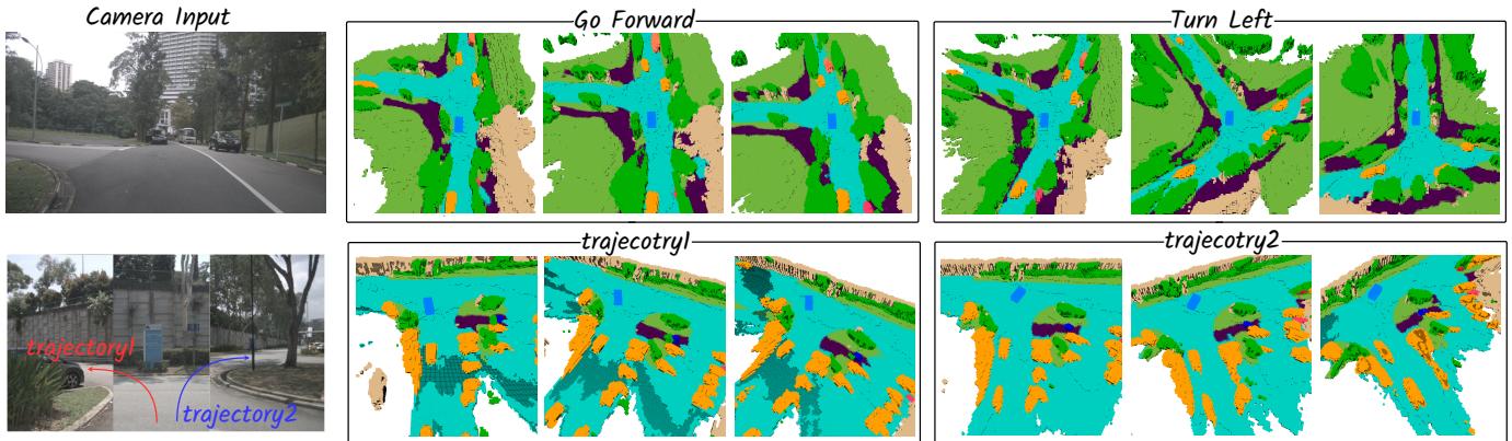
Figure 5: Qualitative results of controllable generation, using the high-level command or low-level trajectory conditions.

Table 4: Planning upper bound when using GT trajectory.

Action Condition	L2(m)↓				Collision (%) ↓
	1s	2s	3s	Avg.	1s	2s	3s	Avg.
GT trajectory	0.26	0.52	0.89	0.56	0.02	0.11	0.36	0.16
Pred trajectory	0.32 0.75		51.49	0.85	0.05	0.17	0.64	0.29

Table 4 shows that using ground-truth trajectories as action conditions yields better planning results than predicted trajectories. However, using predicted trajectories slightly improves occupancy and flow forecasting quality, as indicated by comparisons in Table 3 (line 2 vs. line 7) and supported by Tables 1 and 2, where Drive-OccWorldP outperforms Drive-OccWorldA. This performance gain may stem from planning constraints associated with predicted trajectories, allowing the planner to perform cross-attention between trajectories and BEV features. This process constrains the BEV features to account for ego motion, thereby enhancing perception performance. Additionally, using predicted trajectories during training improves model learning to boost performance during testing.

Additionally, in Figure 5, we demonstrate the capability of Drive-OccWorld to simulate various future occupancies based on specific ego motions, showcasing the potential of Drive-OccWorld as a neural simulator for generating plausible occupancy for autonomous driving.

4.3 End-to-end Planning with Drive-OccWorld

Table 5 presents the planning performance compared to existing end-to-end methods in terms of L2 error and collision rate. We provide results under different evaluation protocol settings from ST-P3 and UniAD. Specifically, NoAvg denotes the result at the corresponding timestamp, while TemAvg calculates metrics by averaging performances from 0.5s to the corresponding timestamp.

As shown in Table 5, Drive-OccWorldP achieves superior planning performance compared to existing methods. For instance, Drive-OccWorldP† obtains relative improvements of $33\%$ , $22\%$ , and $9.7\%$ on $\mathrm{L}2@$ 1s, $\mathrm{L}2@2\mathrm{s}$ , and $\mathrm{L}2@3\mathrm{s}$ , respectively, compared to $\mathrm{UniA}{\mathrm{D}}^{†}$ . We attribute this improvement to the world model’s capacity to accumulate world knowledge and envision future states. It effectively enhances the planning results for future timestamps and improves the safety and robustness of end-to-end planning.

Table 5: End-to-end Planning Performance on nuScenes. † indicates the NoAvg evaluation protocol, while ‡ denotes the TemAvg protocol. ∗ signifies the use of ego status in the planning module and the calculations of collision rates following BEV-Planner (Li et al. 2024b).

Method	L2 (m)↓				Collision (%)↓
	1s	2s3s		Avg.	1s	2s	3s	Avg.
NMP (Zeng et al. 2019)	-	=	2.31		=		1.92		-
SA-NMP (Zeng et al.2019)	-		2.05					1.59	-
FF (Hu et al. 2021) EO (Khurana et al. 2022)	0.551.20 2.54 0.671.36 2.78			1.43 1.60		0.060.17 0.04	0.09	1.07 0.88	0.43 0.33
ST-P3† (Hu et al. 2022)
UniADt (Hu et al.2023b)	1.72 0.48	3.26 0.96	54.86 1.65	3.28 1.03		0.44 0.05	1.08	3.01	1.51
VAD-Base† (Jiang et al. 2023)	0.54	1.15	1.98		1.22	0.10	0.17 0.24	0.71	0.31
OccNet†(Tong et al.2023)	1.29		2.13 2.99	2.14		0.21	0.59	0.96	0.43
Drive-OccWorldPt (Ours)	0.32		0.75 1.49	0.85		0.05		1.37	0.72
								0.17 0.64	0.29
ST-P3* (Hu et al. 2022) UniAD‡ (Hu et al.2023b)	1.33 0.44	2.11	2.90	2.11		0.23	0.62	1.27	0.71
VAD-Base‡ (Jiang et al.2023)		40.67	0.96		0.69		0.040.08	0.23	0.12
Drive-WM* (Wang et al.2024b)	0.41	0.70	1.05		0.72	0.07	0.17	0.41	0.22
Drive-OccWorldP‡ (Ours)	0.43	0.77	1.20		0.80	0.10	0.21	0.48	0.26
		0.25 0.44 0.72		0.47			0.03 0.08 0.22		0.11
UniAD** (Hu et al.2023b)	0.20 0.42
VAD-Base** (Jiang et al.2023)	0.17 0.34		0.75		0.46 0.37			0.02 0.25 0.84	0.37
BEV-Planner** (Li et al.2024b)			0.60			0.04	0.27	0.67	0.33
		0.160.32	0.57		0.35		0.000.290.73		0.34
Drive-OccWorldP‡* (Ours)	0.17	0.31	0.49		0.32		0.020.24 0.62		0.29

Recent studies (Li et al. 2024b) have examined the impact of incorporating ego status into the planning module. In line with this research, we also conduct a fair comparison between our model equipped with ego status and previous works. Our findings indicate that Drive-OccWorld still achieves the highest performance at distant future timestamps, demonstrating the effectiveness of continuous forecasting and planning.

4.4 Ablation Study

The default configuration for the ablation experiments involves using one historical and the current images as input to predict the inflated GMO over two future timestamps.

Conditional Normalization. In Table 6, we ablate the conditional normalization method while discarding the action conditions in Sec. 3.3 to avoid potential influence. The results indicate that each pattern yields gains, particularly with

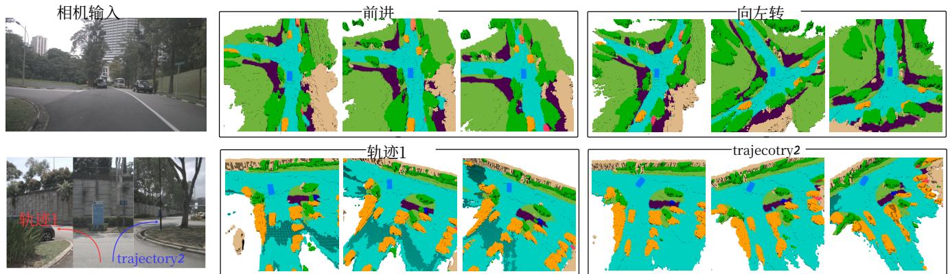
图5：可控生成的定性结果，使用高层次的指令 或低层次的轨迹条件。

动作条件	L2(米）←				碰撞(%) √
	1s	2s	3s	Avg.	1s	2s	3s	Avg.
真实轨迹	0.26	0.52	0.89	0.56	0.02	0.11	0.36	0.16
Pred trajectory	0.32	0.75	1.49	0.85	0.05	0.17	0.64	0.29

表4：在使用真实轨迹时的规划上界。

表4显示，使用真实轨迹作为动作条件比使用预测轨迹能获得更好的规划结果。然而，使用预测轨迹会略微提升占用和流量预测质量，这可以从表3 (第2行 vs.第7行)的比较看出，并由表1 和2支持，其中Drive‑OccWorldP 的表现优于 Drive‑OccWorldA。这种性能提升可能源自与预测轨迹相关的规划约束，使规划器能够在轨迹与 BEV 特征之间执行交叉注意力。该过程约束了 BEV 特征以考虑自车运动，从而增强感知性能。此外，在训练中使用预测轨迹有助于模型学习，从而在测试时提升表现。

此外，在图5中，我们展示了 Drive‑OccWorld 根据特定自车运动模拟各种未来占用的能力，展示了Drive‑OccWorld 作为生成自动驾驶合理占用的神经模拟器的潜力。

4.3 使用 Drive‑OccWorld 的端到端规划

表5 展示了与现有端到端方法在 L2误差和碰撞率方面的规划性能对比。我们在来自 ST‑P3 和 UniAD 的不同评估协议设置下提供结果。具体而言，NoAvg表示对应时间戳的结果，而TemAvg 通过从 0.5秒 到对应时间戳 平均性能来计算评估指标。

如表5所示，Drive‑OccWorldP 在规划性能上优于现有方法。例如，Drive‑OccWorldP† 在 L2@1s、L2$@2s$ 和 $L2@3\mathrm{s}$ 上分别比 UniAD†提高了 $33\%$ 、 $22\%$ 和$9.7\%$ （相对提升）。我们将这一改进归因于世界模型累积世界知识并设想未来状态的能力。它有效提升了对未来时间戳的规划结果，并增强了端到端规划的安全性和鲁棒性。

Method	L2(米）↓ 1s 2s 3s Avg.	碰撞 (%) 1s 2s	↓ 3s Avg.
NMP (Zeng等，2019) SA-NMP (Zeng等，2019) FF (Hu等，2021) EO (Khurana 等人 2022)	= 0.55 1.20 2.54 1 0.67 1.36 2.78 1	2.31 92 2.05 59	[06 0.17 1.07 0.4 04 0.09 0.88 0.3
ST-P3† (Hu等人 2022) UniADt(Hu等人 2023b) VAD-Base† (Jiang 等人 2023) OccNett (Tong 等人 2023) Drive-OccWorldP† (我们的（	1.72 3.26 4.86 3 0.48 0.96 1.65 1 0.54 1.15 1.98 1 1.29 2.13 2.99 2 0.32	0.441.08 3.011 05 0.17 0.710.3 10 0.24 0.96 0.4 21 0.59 1.37 0.7
Ours) ST-P3* (Huetal.2022) 1.33 2.11 2.90 2.11 0.23 UniAD*(Hu et al.2023b) 0.440.67 0.96 0.69 VAD-Base* (Jiangetal.2023)0.410.70 1.05 0. Drive-WM‡ (Wangetal.2024pb) 0.43 0.77 1.2( Drive-OccWorldP‡(我们的（ Qurs))	0.25	1.27 0.71 b.08 0.23 0.12 07 0.17 0.41 0.22 0.10 0.210.48 0
UniAD#* (Hu等人2023b) VAD-Base** (Jiangetal.2023 0.17 0.340.60( BEV-Planner‡*(Li等人2024b)0.160.320.57( Drive-OccWorldP‡*(我们(Ours）)	0.20 0.42 0.75( 0.17	.02 0.25 0.84 0.3 .04 0.27 0.67 0.3 00 0.29 0.73 0.34

表 5： 端到端规划性能 在 nuScenes 上。† 表示 NoAvg 评估协议，而 ‡ 表示 TemAvg 协议。 ∗表示在规划模块中使用自身状态，并按BEV‑Planner (Li 等人 2024b) 计算碰撞率。

近期研究（Li 等人 2024b）考察了将自身状态纳入规划模块的影响。与该研究一致，我们也在本模型中加入自身状态并与以往工作进行了公平比较。结果表明，Drive‑OccWorld 在较远未来时间戳仍然取得最高性能，证明了连续预测和规划的有效性。

4.4 消融研究

默认配置的消融实验包括使用一张历史图像和当前图像作为输入，以预测未来两个时间戳的Inflated GMO。

条件归一化。在表6中，我们在放弃第3.3 节中动作条件以避免潜在影响的同时，对条件归一化方法进行了消融。结果表明每种模式都带来提升，尤其是

Table 6: Ablations on the conditional normalization.

Conditional Normalization semantic ego-motion agent-motion			mIoUcmloUf(1s）mloUf			VPQ
『	√		28.7	26.4	26.8 33.5
		29.0个0.3	26.6+0.2	27.0个0.2	33.2
		29.4个0.7 29.3个0.6	28.3个1.9 27.1个0.7	28.5个1.7 27.5个0.7	32.6 34.4↑0.9
	√	√	29.4个0.7	28.3个1.9	28.6个1.8	|34.5个1.0

Table 7: Ablations on the action conditioning interface.

Condition Interface addition cross-attention		Fourier Embed	mIoUc	mIoUf(1s）1	mIoUf	VPQ
！		√	28.7 28.9年0.2	26.4 27.4个1.0	26.8 28.0个12	33.5 34.2个0.7
	√		28.5	27.1个0.7	27.4个0.6	33.9个0.4
	√	√	29.0 个0.3	27.6个1.2	27.8个1.0	35.0个1.5

ego-motion aware normalization achieving a $1.9\%$ increase in ${\mathrm{mIoU}}_f$ , highlighting the importance of ego status for future state forecasting. Additionally, agent-motion aware normalization enhances ${\mathrm{VQP}}_f^{\ast }$ by $0.9\%$ by compensating for the movements of other agents.

Action Conditioning Interface. In Table 7, we investigate the method of injecting action conditions into the world decoder. Compared to adding conditions to BEV queries, cross-attention is a more effective approach for integrating prior knowledge into the generation process. Furthermore, Fourier embedding provides additional improvement by encoding conditions into latent space at high frequencies.

Occupany-based Costs. Table 8 ablates the occupancybased cost function, and the results indicate that each cost factor contributes to safe planning, particularly highlighting that the absence of agent constraints results in a higher collision rate. Additionally, BEV refinement is vital as it provides more comprehensive 3D information about the environment.

5 Conclusion

We propose Drive-OccWorld, a 4D occupancy forecasting and planning world model for autonomous driving. Flexible action conditions can be injected into the world model for action-controllable generation, facilitating a broader range of downstream applications. An occupancy-based planner is integrated with the world model for motion planning, considering both safety and the 3D structure of the environment. Experiments demonstrate that our method exhibits remarkable performance in occupancy and flow forecasting. Planning results are improved by leveraging the world model’s capacity to accumulate world knowledge and envision future states, thereby enhancing the safety and robustness of end-to-end planning.

Acknowledgments

We thank Jiangning Zhang and Jiang He for helpful discussions and valuable support on the paper. We thank all authors for their contributions. This work was supported by a Grant from The National Natural Science Foundation of China (No. 62103363).

Table 8: Contributions of occupancy-based cost factors.

Cost Factors			BEV	L2(m)↓				Collision (%)↓
		Agent Road Volume		Refine	0.5s 1s	1.5s	Avg.	0.5s	1s	1.5s	Avg.
X	√		√	0.15	0.30	0.50	0.32	10.14	0.16	0.18	0.16
	X	交	√	0.14	0.28	0.46	0.29	0.09	0.11	0.13	0.11
1			√	0.14	0.27	0.44	0.28	0.09	0.14	0.18	0.14
	1	X	×	0.22	0.36	0.52	0.37	0.14	0.20	0.27	0.20
√	√	√	√	0.11	0.26	0.46	0.28	0.04	0.11	0.13	0.09

References

Agro, B.; Sykora, Q.; Casas, S.; Gilles, T.; and Urtasun, R. 2024. UnO: Unsupervised Occupancy Fields for Perception and Forecasting. In Proceedings of the IEEE/CVF Conference on Computer Vision and Pattern Recognition, 14487– 14496.
Ayoub, J.; Zhou, F.; Bao, S.; and Yang, X. J. 2019. From manual driving to automated driving: A review of 10 years of autoui. In Proceedings of the 11th international conference on automotive user interfaces and interactive vehicular applications, 70–90.
Berman, M.; Rannen Triki, A.; and Blaschko, M. B. 2018. The lovasz-softmax loss: A tractable surrogate for the op- ´ timization of the intersection-over-union measure in neural networks. In Proceedings of the IEEE Conference on Computer Vision and Pattern Recognition, 4413–4421.
Blattmann, A.; Dockhorn, T.; Kulal, S.; Mendelevitch, D.; Kilian, M.; Lorenz, D.; Levi, Y.; English, Z.; Voleti, V.; Letts, A.; et al. 2023. Stable video diffusion: Scaling latent video diffusion models to large datasets. arXiv preprint arXiv:2311.15127.
Boeder, S.; Gigengack, F.; and Risse, B. 2024. OccFlowNet: Towards Self-supervised Occupancy Estimation via Differentiable Rendering and Occupancy Flow. arXiv preprint arXiv:2402.12792.
Caesar, H.; Bankiti, V.; Lang, A. H.; Vora, S.; Liong, V. E.; Xu, Q.; Krishnan, A.; Pan, Y.; Baldan, G.; and Beijbom, O. 2020. nuscenes: A multimodal dataset for autonomous driving. In Proceedings of the IEEE/CVF conference on computer vision and pattern recognition, 11621–11631.
Cao, A.-Q.; and de Charette, R. 2022. Monoscene: Monocular 3d semantic scene completion. In Proceedings of the IEEE/CVF Conference on Computer Vision and Pattern Recognition, 3991–4001.
Chen, L.; Li, Y.; Huang, C.; Xing, Y.; Tian, D.; Li, L.; Hu, Z.; Teng, S.; Lv, C.; Wang, J.; et al. 2023. Milestones in autonomous driving and intelligent vehicles—Part I: Control, computing system design, communication, HD map, testing, and human behaviors. IEEE Transactions on Systems, Man, and Cybernetics: Systems, 53(9): 5831–5847.
Doll, S.; Hanselmann, N.; Schneider, L.; Schulz, R.; Cordts, M.; Enzweiler, M.; and Lensch, H. 2024. DualAD: Disentangling the Dynamic and Static World for End-to-End Driving. In Proceedings of the IEEE/CVF Conference on Computer Vision and Pattern Recognition, 14728–14737.
Gao, S.; Yang, J.; Chen, L.; Chitta, K.; Qiu, Y.; Geiger, A.; Zhang, J.; and Li, H. 2024. Vista: A Generalizable Driving

条件归一化 语义自我运动主体运动		mIoUe	mIoUf (1 s)	mIoUf ~	VPQ
√ ！		28.7	26.4	26.8	33.5
		29.0个0.3	26.6+0.2	27.0个0.2	33.2
	√	29.4个0.7 29.3个0.6	28.3†1.9 27.1个0.7	28.5个1.7 27.50.7	32.6 34.4+0.9
?	√ √	29.4个0.7	28.3个1.9	28.6个18	34.5个1.0

表6：关于条件归一化的消融实验。

条件接口 addition交叉注意力入	傅里叶	mIoUc	mIoUf (1 s)	~ mIoUf	VPQ
√ √	【	28.7 28.9个0.2 28.5	26.4 27.4个1.0	26.8 28.0个1.2	33.5 34.2年0.7
√	√	29.0个0.3	27.1个0.7 27.6↑1.2	27.4个0.6 27.8个1.0	33.9年0.4

表7：关于动作条件接口的消融实验。

自我运动感知归一化在mIoUf上实现了 $1.9\%$ 的提升，突显了自身状态对未来状态预测的重要性。此外，主体运动感知归一化通过补偿其他智能体的运动，使 ${\mathrm{VQP}}_f^{\ast }$ 提升了$0.9{\%}_{{\text{ 0 }}_{\text{ 0 }}}$ 。

动作条件接口。在表7中，我们研究了将动作条件注入世界解码器的方法。与将条件添加到BEV查询相比，交叉注意力是将先验知识融入生成过程的更有效方法。此外，傅里叶嵌入通过在潜在空间的高频部分编码条件，带来了额外的改进。

基于占用的代价。表8 对基于占用的代价函数进行了消融，结果表明每个代价因子都有助于安全规划，特别是缺少智能体约束会导致更高的碰撞率。此外，BEV精化非常重要，因为它提供了关于环境的更全面的三维信息。

5 结论

我们提出了 Drive‑OccWorld，一种用于自动驾驶的4D 占据 预测与 规划世界模型。灵活的动作条件可以注入到世界模型中以实现可控动作生成，从而促进更广泛的下游应用。基于占据的规划器与世界模型集成，用于运动规划，兼顾安全性和环境的三维结构。实验证明，我们的方法在占据和流量预测方面表现出显著的性能。通过利用世界模型积累世界知识并预见未来状态的能力，规划结果得到了改进，从而提升了端到端规划的安全性和鲁棒性。

致谢

我们感谢 Jiangning Zhang 和 Jiang He 在论文撰写过程中提供的有益讨论和宝贵支持。我们感谢所有作者的贡献。本工作由中国国家自然科学基金委员会资助（项目编号：62103363） 。

代价因子 智能体道路体积		BEV 0.5秒精化	L2(米）↓			碰撞（%） ↓
				1s1.5s	平均值0.5秒	1s 1.5s	Avg.
区			√	0.150.30 0.50	0.32	0.14 0.16 0.18	0.16
	X		、	0.14 0.28 0.46	0.29	0.09 0.110.13	0.11
：	：		√	0.14 0.27 0.44	0.28	0.09 0.14 0.18	0.14
			X	0.22 0.36 0.52	0.37	0.140.200.27	0.20
√	√	√	√	0.11	0.28	0.040.11 0.13	0.09

表 8：基于占用的成本因素的贡献。

参考文献
Agro, B.; Sykora, Q.; Casas, S.; Gilles, T.; and Urtasun, R. 2024. UnO: Unsupervised Occupancy Fields for Perception and Forecasting. In Proceedings of the IEEE/CVF Conference on Computer Vision and Pattern Recognition, 14487– 14496.
Ayoub, J.; Zhou, F.; Bao, S.; and Yang, X. J. 2019. From manual driving to automated driving: A review of 10 years of autoui. In Proceedings of the 11th international conference on automotive user interfaces and interactive vehicular applications, 70–90.
Berman, M.; Rannen Triki, A.; and Blaschko, M. B. 2018. The lova´sz-softmax loss: A tractable surrogate for the optimization of the intersection-over-union measure in neural networks. In Proceedings of the IEEE Conference on Computer Vision and Pattern Recognition, 4413–4421.
Blattmann, A.; Dockhorn, T.; Kulal, S.; Mendelevitch, D.; Kilian, M.; Lorenz, D.; Levi, Y.; English, Z.; Voleti, V.; Letts, A.; et al. 2023. Stable video diffusion: Scaling latent video diffusion models to large datasets. arXiv preprint arXiv:2311.15127.
Boeder, S.; Gigengack, F.; and Risse, B. 2024. OccFlowNet: Towards Self-supervised Occupancy Estimation via Differentiable Rendering and Occupancy Flow. arXiv preprint arXiv:2402.12792.
Caesar, H.; Bankiti, V.; Lang, A. H.; Vora, S.; Liong, V. E.; Xu, Q.; Krishnan, A.; Pan, Y.; Baldan, G.; and Beijbom, O. 2020. nuscenes: A multimodal dataset for autonomous driving. In Proceedings of the IEEE/CVF conference on computer vision and pattern recognition, 11621–11631.
Cao, A.-Q.; and de Charette, R. 2022. Monoscene: Monocular 3d semantic scene completion. In Proceedings of the IEEE/CVF Conference on Computer Vision and Pattern Recognition, 3991–4001.
Chen, L.; Li, Y.; Huang, C.; Xing, Y.; Tian, D.; Li, L.; Hu, Z.; Teng, S.; Lv, C.; Wang, J.; et al. 2023. Milestones in autonomous driving and intelligent vehicles—Part I: Control, computing system design, communication, HD map, testing, and human behaviors. IEEE Transactions on Systems, Man, and Cybernetics: Systems, 53(9): 5831–5847.
Doll, S.; Hanselmann, N.; Schneider, L.; Schulz, R.; Cordts, M.; Enzweiler, M.; and Lensch, H. 2024. DualAD: Disentangling the Dynamic and Static World for End-to-End Driving. In Proceedings of the IEEE/CVF Conference on Computer Vision and Pattern Recognition, 14728–14737.
Gao, S.; Yang, J.; Chen, L.; Chitta, K.; Qiu, Y.; Geiger, A.; Zhang, J.; and Li, H. 2024. Vista: A Generalizable Driving

Driving in the Occupancy World: Vision-Centric 4D Occupancy Forecasting and Planning via World Models for Autonomous Driving

Supplementary Material

Contents

A Additional Related Works 12

A.1 End-to-end Autonomous Driving . . . . 12
A.2 Occupancy Prediction and Forecasting . . . 12

Additional Method Details 13

B.1 World Decoder 13
B.2 Loss Function 13

C Experimental Settings 13

C.1 Dataset 13
C.2 Metrics 13
C.3 Implementation Details 14

D Additional Experiments 14

D.1 Effectiveness and Efficiency 14
D.2 Semantic-Conditional Normalization . . . 14
D.3 Semantic Loss . 15

E Additional Visualizations 15

E.1 Action Controllability . . . . . 15
E.2 4D Occupancy Forecasting 18
E.3 Trajectory Planning . . . 18

A Additional Related Works

A.1 End-to-end Autonomous Driving

In recent decades, autonomous driving (AD) algorithms (Ayoub et al. 2019; Chen et al. 2023; Mei et al. 2023b) have significantly advanced from modular pipelines (Guo et al. 2023; Li et al. 2023b) to end-to-end models (Hu et al. 2023b; Jiang et al. 2023), which predict planning trajectories directly from raw sensor data in a unified manner. For instance, P3 (Sadat et al. 2020) and ST-P3 (Hu et al. 2022) learn a differentiable occupancy representation from the perception module, serving as a cost factor for producing safe maneuvers. Building on the success of detection (Huang et al. 2021; Li et al. 2023c,d, 2022; Wang et al. 2023a; Li et al. 2024a) and segmentation $\mathrm{Ng}$ et al. 2020; Peng et al. 2023) in Bird’s-eye view (BEV), several methods plan trajectories based on BEV perception and prediction. UniAD (Hu et al. 2023b) is a representative planningoriented end-to-end model that integrates BEV tracking and motion prediction with planning. VAD (Jiang et al. 2023) employs a vectorized representation in BEV for scene learning and planning. GraphAD (Zhang et al. 2024b) utilizes a graph model to establish interactions among agents and map elements. DualAD (Doll et al. 2024) disentangles dynamic and static representations using object and BEV queries to address the effects of object motion. UAD (Guo et al. 2024) proposes an unsupervised proxy to reduce the need for costly annotations across multiple modules. PARA-Drive (Weng et al. 2024) explores module connectivity and introduces a fully parallel architecture. SparseAD (Zhang et al. 2024a) and SparseDrive (Sun et al. 2024) investigate sparse representations to enhance the efficacy and efficiency of end-toend methods.

A.2 Occupancy Prediction and Forecasting

Occupancy Prediction aims to construct the occupancy state of the surrounding environment based on observations. Existing methods are primarily classified into LiDARbased and camera-based approaches, depending on the input modality.

LiDAR-based methods (Song et al. 2017; Roldao, ˜ de Charette, and Verroust-Blondet 2020; Yan et al. 2021; Yang et al. 2021; Mei et al. 2023a) derive occupancy predictions primarily from grids generated by sparse LiDAR points, investigating the relationships between semantic segmentation and scene completion. In contrast, camera-based methods (Cao and de Charette 2022; Li et al. $2023\mathrm{e}$ ; Wei et al. 2023b; Wang et al. 2023c; Mei et al. 2023c) focus on efficiently transforming 2D image features into 3D representations. For example, TPVFormer (Huang et al. 2023) introduces a tri-perspective view (TPV) representation to describe the 3D structure, OccFormer (Zhang, Zhu, and Du 2023) employs depth prediction for image-to-3D transformation, and Occ3D (Tian et al. 2023) utilizes cross-attention to aggregate 2D features into 3D space. Recent methods (Huang et al. 2024; Zhang et al. 2023a; Boeder, Gigengack, and Risse 2024) also implement occupancy prediction in a self-supervised manner, utilizing neural rendering to convert occupancy fields into depth maps, which can then be supervised using multi-frame photometric consistency.

Occupancy Forecasting aims to predict the near-future occupancy state (i.e., how the surroundings evolve) based on historical and current observations. Existing methods (Khurana et al. 2022, 2023; Toyungyernsub et al. 2022) primarily utilize LiDAR point clouds to identify changes in the surrounding structure and predict future states. For example, Khurana et al. (Khurana et al. 2022) propose a differentiable depth rendering method that generates point clouds from 4D occupancy predictions, facilitating occupancy forecasting training with unannotated LiDAR sequences. Other point cloud prediction methods (Lu et al. 2021; Mersch et al. 2022; Luo et al. 2023) directly forecast future laser points, which can then be voxelized for subsequent occupancy estimation. Cam4DOcc (Ma et al. 2024b) is the first framework for camera-based 4D occupancy forecasting, establishing a benchmark that provides sequential occupancy states for both movable and static objects, along with their 3D backward centripetal flow.

The aforementioned methods can only predict future occupancy states using historical observations. In this work, we propose a framework that simultaneously predicts future occupancy and generates planning trajectories based on

Supplementary Material

Contents

A AdditionalRelated Works 12A.1 End‑to‑end Autonomous Driving . . . . . . 12 A.2 Occupancy Prediction and Forecasting . . . 12B Additional MethodDetails 13B.1 World Decoder.13 B.2 Loss Function.13C ExperimentalSettings 13C.1 Dataset.13 C.2 Metrics.13 C.3 Implementation Details.14D AdditionalExperiments 14D.1 Effectiveness and Efficiency . . . . . 14 D.2 Semantic‑Conditional Normalization . . . . 14 D.3 Semantic Loss.15E AdditionalVisualizations 15E.1 Action Controllability.15 E.2 4D Occupancy Forecasting.18 E.3 Trajectory Planning.18

A 其他相关工作

A.1 端到端自动驾驶

近几十年来，自动驾驶（AD）算法（Ayoub 等人 2019；Chen 等人 2023；Mei 等人 2023b）已从模块化流水线（Guo 等人 2023；Li 等人 2023b）显著发展到端到端模型（Hu 等人 2023b；Jiang 等人 2023），这些模型以统一方式直接从原始传感器数据预测规划轨迹。例如，P3（Sadat等人 2020）和 ST‑P3（Hu 等人 2022）从感知模块学习可微分的占用表示，作为生成安全机动的代价因子。基于鸟瞰图（BEV）中检测（Huang 等人 2021；Li 等人 2023c,d,2022；Wang 等人 2023a；Li 等人 2024a）和分割（Ng 等人 2020；Peng 等人 2023）的成功，若干方法基于 BEV 感知与预测来规划轨迹。UniAD（Hu 等人 2023b）是一个代表性的面向规划的端到端模型，将 BEV 跟踪和运动预测与规划集成在一起。VAD（Jiang 等人 2023）在 BEV 中采用向量化表示进行场景学习和规划。GraphAD（Zhang 等人2024b）利用图模型建立智能体与地图要素之间的交互。DualAD（Doll 等人 2024）通过使用对象查询和 BEV 查询将动态与静态表示解耦，以应对对象运动的影响。UAD（Guo 等人 2024）提出了一种无监督代理以减少多个模块上昂贵标注的需求。PARA‑Drive（Weng 等人 2024）探索了模块连接性并引入了一个

全并行架构。SparseAD (Zhang 等人 2024a) 和SparseDrive (Sun 等人 2024) 研究稀疏表示，以提高端到端方法的有效性和效率。

A.2 占用预测与预测

OccupancyPrediction 旨在基于观测构建周围环境的占用状态。现有方法主要根据输入模态分为基于LiDAR 的方法和基于摄像头的方法。

基于 LiDAR 的方法 (Song et al. 2017; Rold˜ao, de Charette,and Verroust‑Blondet 2020; Yan et al. 2021; Yang et al. 2021;Mei et al. 2023a) 推导占用预这些预测主要来自由稀疏 LiDAR 点生成的网格，研究语义分割与场景补全之间的关系。相对地，基于相机的方法（Cao 和 de Charette 2022；Li 等人 2023e；Wei 等人2023b；Wang 等人 2023c；Mei 等人 2023c）侧重于将二维图像特征高效地转换为三维表示。例如，TPVFormer（Huang 等人 2023）引入了三视角表示（TPV）来描述三维结构，OccFormer（Zhang、Zhu 和 Du 2023）采用深度预测进行图像到三维的转换，Occ3D（Tian 等人 2023）利用交叉注意力将二维特征聚合到三维空间。最近的方法（Huang 等人 2024；Zhang 等人 2023a；Boeder、Gigengack 和 Risse 2024）也以自监督方式实现占用预测，使用神经渲染将占据场转换为深度图，然后可以利用多帧光度一致性进行监督。

占用预测旨在根据历史与当前观测预测近期的占用状态（即，周围环境如何演变）。现有方法（Khurana 等人2022、2023；Toyungyernsub 等人 2022）主要利用LiDAR 点云来识别周围结构的变化并预测未来状态。例如，Khurana 等人（Khurana 等人 2022）提出了一种可微分的深度渲染方法，该方法从四维占用预测生成点云，促进了利用无标注激光雷达序列进行占用预测的训练。其他点云预测方法（Lu 等人 2021；Mersch 等人 2022；Luo 等，2023）直接预测未来的激光点，然后可以将其体素化以便后续的占用估计。Cam4DOcc（Ma et al.2024b）是首个基于相机的4D 占据预测框架，建立了一个基准，提供了可移动和静态对象的序列占据状态及其三维反向向心流。

上述方法只能使用历史观测来预测未来的占用状态。在本工作中，我们提出了一个框架，该框架在预测未来占用的同时，基于占用状态生成规划轨迹

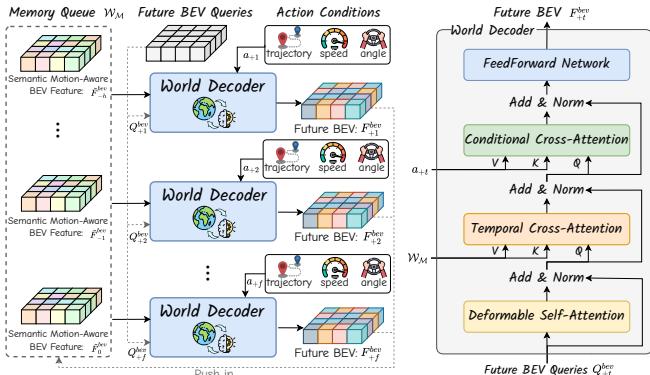
Figure 6: Detailed structure of the world decoder, which predicts the next BEV features based on historical BEV features and expected ego actions in an autoregressive manner.

the occupancy status. Additionally, we implement actionconditioned occupancy generation to associate future predictions with various ego actions.

B Additional Method Details

B.1 World Decoder

As depicted in Figure 6, the world decoder ${\mathcal{W}}_{\mathcal{D}}$ predicts the BEV embeddings at the next timestamp based on historical BEV features stored in $w_{\mathcal{M}}$ and expected action conditions in an autoregressive manner.

Specifically, the learnable BEV queries $Q\in {\mathbb{R}}^{h\times w\times c}$ first perform deformable self-attention to establish contextual relationships. A temporal cross-attention layer is then employed to extract corresponding features from multi-frame historical embeddings. To save memory while maintaining efficiency, this layer also operates in a deformable manner. Notably, the movement of the ego vehicle can cause misalignment between BEV embeddings at different timestamps; thus, reference coordinates are calculated using ego transformations for feature alignment. Subsequently, a conditional cross-attention layer is utilized to perform crossattention between the BEV queries and conditional embeddings, injecting action conditions into the forecasting process. Finally, a feedforward network outputs the generated BEV features, which can be used for future occupancy and flow forecasting.

B.2 Loss Function

We optimize Drive-OccWorld with historical normalization, future forecasting, and trajectory planning in an end-to-end manner by leveraging the following loss functions:

$$\mathcal{L}={\mathcal{L}}_{norm}+{\mathcal{L}}_{fcst}+{\mathcal{L}}_{plan}$$

Normalization Loss. In semantic-conditional normalization, we employ cross-entropy loss to supervise the historical semantic probabilities $S_{-h:0}$ , thereby learning effective semantics for affine transformation. Additionally, $l_1$ loss is used to supervise the historical 3D backward centripetal flow predictions ${\mathcal{F}}_{-h:0}$ . These losses are combined to form the normalization loss ${\mathcal{L}}_{norm}$ , which enhances both semantic and dynamic representations in the historical memories.

Forecasting Loss. For the future forecasting loss ${\mathcal{L}}_{fcst}$ , flow predictions ${\mathcal{F}}_{1:f}$ are supervised using $l_1$ loss, while occupancy predictions ${\mathcal{S}}_{1:f}$ are constrained by multiple losses, including cross-entropy loss ${\mathcal{L}}_{ce}$ , Lovasz loss ´ ${\mathcal{L}}_{lovasz}$ , and binary occupancy loss ${\mathcal{L}}_{bce}$ :

$${\mathcal{L}}_{occ}=\frac{1}{N_f}\sum _{t=1}^{N_f}({\mathcal{L}}_{ce}(S_t,{\hat{S}}_t)+{\mathcal{L}}_{lovasz}(S_t,{\hat{S}}_t)+{\mathcal{L}}_{bce}({\mathcal{O}}_t,{\hat{\mathcal{O}}}_t))$$

where $N_f$ denotes the number of future frames, ${\hat{S}}_t$ represents the ground-truth semantic occupancy at timestamp $t$ , and $\mathcal{O}$ is the binary occupancy. These losses are combined to constrain the semantics and geometries of occupancy forecasting, guiding Drive-OccWorld in learning how the world evolves.

Planning Loss. Since selecting the lowest-cost trajectory from a discrete set ${\tau }^{\ast }$ is not differentiable, we employ a maxmargin loss inspired by ST-P3 (Sadat et al. 2020; Hu et al. 2022) to penalize trajectory candidates with low costs that deviate from the expert trajectory. Let $o$ represent the occupied grids by agents and roads, and let $\hat{\tau }$ denote the expert trajectory. The max-margin loss encourages the expert trajectory to have a smaller occupancy cost than other candidates.

Overall, the planning loss consists of three components: the max-margin loss, a naive $l_2$ loss for imitation learning, and a collision loss $l_{coll}$ that ensures the planned trajectory avoids grids occupied by obstacles:

$${\mathcal{L}}_{plan}=\underset{{\tau }^{\ast }}{\max }[f_o(o,\hat{\tau })-f_o(o,{\tau }^{\ast }){]}_{+}+l_2({\tau }_o,\hat{\tau })+l_{coll}({\tau }_o,a)$$

where $f_o$ is the occupancy-based cost function, ${\tau }_o$ denotes the final predicted trajectory, $a$ represents the grids occupied by obstacles, and $[\cdot {]}_{+}$ denotes the ReLU function.

C Experimental Settings

C.1 Dataset

We adopt the nuScenes (Caesar et al. 2020), nuScenesOccupancy (Wang et al. 2023c), and Lyft-Level5 datasets for occupancy forecasting and planning. Following Cam4DOcc (Ma et al. 2024b), we use the corresponding images from two historical frames and one current frame as input to predict future states over four timestamps. Since nuScenes is annotated at 2Hz while Lyft-Level5 is annotated at 5Hz, we report the results with 2s and 0.8s time intervals, respectively. After reorganizing the data, the number of sequences for training and testing is 23,930 and 5,119 in scenes and 15,720 and 5,880 in Lyft-Level5.

C.2 Metrics

Occupancy Forecasting is evaluated using the mIoU metric, with ${\mathrm{mIoU}}_c$ and ${\mathrm{mIoU}}_f$ denoting the performances of the current and future timestamps, respectively:

$${\mathrm{mIoU}}_c({\mathcal{S}}_c,{\hat{\mathcal{S}}}_c)=\frac{{\sum }_{H,W,L}{\mathcal{S}}_c\cdot {\hat{\mathcal{S}}}_c}{{\sum }_{H,W,L}{\mathcal{S}}_c+{\hat{\mathcal{S}}}_c-{\mathcal{S}}_c\cdot {\hat{\mathcal{S}}}_c}$$

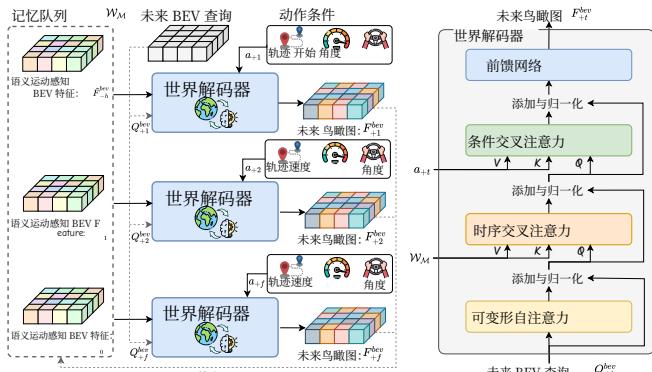
图 6：世界解码器的详细结构，该结构以自回归方式基于历史 BEV 特征和预期自车动作预测下一个 BEV 特征。

此外，我们实现了动作条件占用生成，以将未来预测与各种自车动作关联起来。

B 其他方法细节

B.1 世界解码器

如图 6 所示，世界解码器 ${\mathcal{W}}_{\mathcal{D}}$ 以自回归方式根据存储在 $w_{\mathcal{M}}$ 中的历史鸟瞰视图特征和预期动作条件预测下一个时间戳的鸟瞰视图嵌入。

具体而言，可学习的鸟瞰视图查询 $Q\in {\mathbb{R}}^{h\times w\times c}$ 首先执行可变形自注意力以建立上下文关系。然后使用时序交叉注意力层从多帧历史嵌入中提取对应特征。为在保持效率的同时节省内存，该层也以可变形方式运行。值得注意的是，自车的移动会导致不同时间戳的鸟瞰视图嵌入错位；因此使用自车变换计算参考坐标以进行特征对齐。随后，使用条件交叉注意力层在鸟瞰视图查询与条件嵌入之间执行交叉注意力，将动作条件注入预测过程中。最后，前馈网络输出生成的鸟瞰视图特征，可用于未来占用和流量预测。

B.2 损失函数

我们通过以下损失函数，以端到端的方式对 Drive‑OccWorld 进行历史归一化、未来预测和轨迹规划的联合优化：

$$\mathcal{L}={\mathcal{L}}_{norm}+{\mathcal{L}}_{fcst}+{\mathcal{L}}_{plan}$$

归一化损失。在语义条件归一化中，我们使用交叉熵损失来监督历史语义概率 $ { \mathcal { S } } _ { - h : 0 }$ ，从而为仿射变换学习有效的语义表示。此外， $l_1$ 损失用于监督历史三维反向向心流预测 ${\mathcal{F}}_{-h:00}$ 。这些损失被组合形成归一化损失${\mathcal{L}}_{norm}$ ，以增强历史记忆中的语义和动态表示。

预测损失。 对于未来预测损失 ${\mathcal{L}}_{fcst}$ ，流预测 ${\mathcal{F}}_{1:f}$ 使用 $l_1$ 损失进行监督，而占用预测 ${\mathcal{S}}_{1:f}$ 则受多个损失约束，包括交叉熵损失 ${\mathcal{L}}_{ce}$ 、Lov´asz损失 ${\mathcal{L}}_{lovasz}$ 和二值占用损失 ${\mathcal{L}}_{bce}$ ：

$${\mathcal{L}}_{occ}=\frac{1}{N_f}\sum _{t=1}^{N_f}({\mathcal{L}}_{ce}(S_t,{\hat{S}}_t)+{\mathcal{L}}_{lovasz}(S_t,{\hat{S}}_t)+{\mathcal{L}}_{bce}({\mathcal{O}}_t,{\hat{\mathcal{O}}}_t))$$

ˆ 其中 $N_f$ 表示未来帧的数量， $S_t$ 表示时间戳 $t$ 时的真实语义占用， $\mathcal{O}$ 为二值占用。这些损失共同约束占用预测的语义和几何，指导 Drive‑OccWorld 学习世界如何演化。

规划损失。 由于从离散集合 ${\tau }^{\ast }$ 中选择最低代价轨迹不可微分，我们采用受 ST‑P3 (Sadat 等人 2020；Hu 等人 2022) 启发的最大间隔损失，对那些代价低但偏离专家轨迹的轨迹候选进行惩罚。令 $o$ 表示由智能体和道路占据的网格，令 ${\hat{\xi }}_{\tau }$ 表示专家轨迹。最大间隔损失鼓励专家轨迹的占用代价比其他候选更小。

总体而言，规划损失由三部分组成：最大间隔损失、用于模仿学习的朴素 $l_2$ 损失，以及确保规划轨迹避开被障碍物占据网格的碰撞损失 $l_{coll}$ ：

$${\mathcal{L}}_{plan}=\underset{{\tau }^{\ast }}{\max }[f_o(o,\hat{\tau })-f_o(o,{\tau }^{\ast }){]}_{+}+l_2({\tau }_o,\hat{\tau })+l_{coll}({\tau }_o,a)$$

其中 $f_o$ 是基于占用的代价函数， ${\tau }_o$ 表示最终预测轨迹，$a$ 代表被障碍物占据的网格，且 $[\cdot {]}_{+}$ 表示ReLU函数。

C 实验设置

C.1 数据集

我们采用 nuScenes (Caesar 等人 2020)、
nuScenes‑Occupancy (Wang 等人 2023c) 和 Lyft‑Level5 数据集用于占用预测与规划。按照 Cam4DOcc (Ma 等人 2024b) 的做法，我们使用来自两帧历史帧和一帧当前帧的对应图像作为输入，以预测未来四个时间戳的未来状态。由于
nuScenes 的注释为 2Hz 而 Lyft‑Level5 为 5Hz，我们分别以2秒 和 $0.8\hslash \gg$ 的时间间隔报告结果。重组数据后，scenes 中训练和测试的序列数分别为 23,930 和 5,119，在 Lyft‑Level5 中分别为 15,720 和 5,880。

C.2 评估指标

OccupancyForecasting 的评估采用 themIoU 指标，mIoUc和 mIoUf 分别表示当前时间戳和未来时间戳的性能：

$${\mathrm{mIoU}}_c({\mathcal{S}}_c,{\hat{\mathcal{S}}}_c)=\frac{{\sum }_{H,W,L}{\mathcal{S}}_c\cdot {\hat{\mathcal{S}}}_c}{{\sum }_{H,W,L}{\mathcal{S}}_c+{\hat{\mathcal{S}}}_c-{\mathcal{S}}_c\cdot {\hat{\mathcal{S}}}_c}$$

$${\mathrm{mIoU}}_f(S_f,{\hat{S}}_f)=\frac{1}{N_f}\sum _{t=1}^{N_f}\frac{{\sum }_{H,W,L}{S}_t\cdot {\hat{S}}_t}{{\sum }_{H,W,L}{S}_t+{\hat{S}}_t-S_t\cdot {\hat{S}}_t}$$

where $S_t$ and ${\hat{S}}_t$ represent the predicted and ground-truth semantic occupancy at timestamp $t$ , respectively. Here, $H$ , $W$ , and $L$ denote the dimensions of the 3D volume, while $N_f$ represents the number of future frames.

Additionally, we introduce a quantitative indicator ${\widetilde{\mathrm{mIoU}}}_f$ , weighted by timestamp, based on the principle that occupancy predictions at nearby timestamps are more critical for planning:

$$\mathrm{m}{\widetilde{\mathrm{Io}}\mathrm{U}}_f(S_f,{\hat{S}}_f)=\frac{1}{N_f}\sum _{t=1}^{N_f}\frac{1}{t}\sum _{k=1}^t\frac{{\sum }_{H,W,L}{S}_k\cdot {\hat{S}}_k}{{\sum }_{H,W,L}{S}_k+{\hat{S}}_k-S_k\cdot {\hat{S}}_k}$$

Flow Forecasting is evaluated by extending the video panoptic quality (VPQ) metric (Kim et al. 2020) from 2D instance prediction to 3D instance prediction. Specifically, instance centers are determined from occupancy predictions at $t=0$ using non-maximum suppression (NMS), and voxelwise instance IDs are assigned using the predicted 3D backward centripetal flow over $t\in [1,\bar{f}]$ . Since instance centers may be duplicated during the NMS operation, we introduce a simple yet efficient center clustering technique that combines the center proposals based on their relative distances, merging them into a more unified set. The ${\mathrm{VPQ}}_f$ can be calculated as follows:

$$\nabla {\mathrm{PQ}}_f({\mathcal{F}}_f,{\hat{\mathcal{F}}}_f)=\frac{1}{N_f}\sum _{t=0}^{N_f}\frac{{\sum }_{(p_t,q_t)\in T{P}_t}\mathrm{IoU}(p_t,q_t)}{|T{P}_t|+\frac{1}{2}|F{P}_t|+\frac{1}{2}|F{N}_t|}$$

where $|T{P}_t|,|F{P}_t|$ , and $|F{N}_t|$ represent the true positives, false positives, and false negatives at timestamp $t$ , respectively. Following Cam4DOcc, a predicted instance is considered a true positive if its IoU is greater than 0.2 and the corresponding instance ID is correctly tracked.

Planning is evaluated using L2 error and collision rate at various timestamps. We also report the modified collision rate proposed in (Li et al. 2024b), where the collisions at each moment depend on previous timestamps:

$$CR(t)=\sum _{t=0}^{N_f}{\mathbb{I}}_t>0$$

where ${\mathbb{I}}_t$ indicates whether the ego vehicle at timestamp $t$ will intersect with other obstacles.

C.3 Implementation Details

The 3D environment is voxelized within $[[\pm 51.2\mathrm{m}],[\pm 51.2\mathrm{m}],[-5\mathrm{m},3\mathrm{m}]]$ at a voxel resolution of $0.2\mathrm{m}$ , resulting in a volume size of $512\times 512\times 40$ . The historical encoder ${\mathcal{W}}_{\mathcal{E}}$ is derived from the BEVFormerbased encoder (Li et al. 2022), which includes an image backbone with a Feature Pyramid Network (FPN) neck and six additional transformer encoder layers. The spatial resolutions of BEV queries are set to $h,w=200$ . The world decoder ${\mathcal{W}}_{\mathcal{D}}$ consists of three layers, each with 256 channels. The prediction heads have output channels set to 16 to convert BEV embeddings into 3D semantic occupancy and flow predictions $(S,\mathcal{F})\stackrel{⌣}{\in }{\mathbb{R}}^{200\times 200\times 16}$ . During training, we use historical multi-view camera images over two timesteps to forecast future occupancy over two seconds (with each timestep corresponding to a 0.5-second interval). We employ an AdamW optimizer with an initial learning rate of $\bar{2}\times 10^{-4}$ and a cosine annealing scheduler to train Drive-OccWorld on 8 NVIDIA A100 GPUs.

Table 9: Latency and performance based on varying numbers of input frames and memory queue lengths. Latency measurements are conducted on an A6000 GPU.

No.of Frames History	Current	Memory Length	mIoUc	mIoUf (2 s)	）mloUf	Latency (ms)
						Wε	WM	WD
0	1	1	13.0	12.1	12.3	140	10	190
1	1	1	14.3个1.3	13.4个1.3	13.6个1.3	269	12	188
2	1	2	14.8个1.8	13.8个1.7	14.1个1.8	406	19	207
2	1	3	15.1个2.1	14.1 ↑2.0	14.3个2.0	401	26	220

Table 10: Ablation studies on the semantic occupancy loss functions, utilizing one historical and the current inputs to predict future states across two timestamps.

Semantic Loss Cross Entropy Binary Occupancy Lovasz		mIoU。mIoUf(1s) mloUf				VPQ
√		28.3	27.2	27.5	34.1
√	√	28.7↑0.4	27.9个0.7	28.1↑0.6	34.3↑0.2
√	√	29.4个1.1	28.3个1.1	28.6个1.1	34.5个0.4

D Additional Experiments

D.1 Effectiveness and Efficiency

In Table 9, we compare the performance and latency of different configurations based on the number of input frames and the length of the memory queue. We observe that without historical inputs, the performance at the current moment, ${\mathrm{mIoU}}_c$ , is slightly weaker. However, it can still generate plausible future forecasting results while operating at real-time speed. Furthermore, increasing both the number of input frames and the length of the memory queue leads to improvements in performance.

Regarding latency, most of the time consumption is attributed to the historical encoder ${\mathcal{W}}_{\mathcal{E}}$ . In contrast, the memory queue $w_{\mathcal{M}}$ and the world decoder ${\mathcal{W}}_{\mathcal{D}}$ exhibit limited latency, even as the number of input frames increases, demonstrating the efficiency of our architectural design. We further test the latencies of the modules in ${\mathcal{W}}_{\mathcal{E}}$ , where the image backbone runs at $27\mathrm{ms}$ , the FPN neck runs at 13 ms, and the transformer encoder runs at $100\mathrm{ms}$ . In future work, we will explore sparse representations such as SparseBEV (Liu et al. 2023) to enhance the efficacy and efficiency of Drive-OccWorld.

D.2 Semantic-Conditional Normalization

The original BEV embeddings are derived from 2D image features and exhibit ray-shaped patterns, as shown in the visualizations of Before Normalization in Figure 7. This phenomenon can be explained by the fact that waypoints along

$${\mathrm{mIoU}}_f({\mathcal{S}}_f,{\hat{\mathcal{S}}}_f)=\frac{1}{N_f}\sum _{t=1}^{N_f}\frac{{\sum }_{H,W,L}{\mathcal{S}}_t\cdot {\hat{\mathcal{S}}}_t}{{\sum }_{H,W,L}{\mathcal{S}}_t+{\hat{\mathcal{S}}}_t-{\mathcal{S}}_t\cdot {\hat{\mathcal{S}}}_t}$$

ˆ其中 $S_t$ 和 $S_t$ 分别表示时间戳 $t$ 处的预测语义占用和真实语义占用。这里， $H,W$ 和 $L$ 表示三维体素空间的维度， $N_f$ 表示未来帧数。

此外，我们引入了一个量化指标 $\tilde{\mathbf{m}}\mathbf{IoU}f$ ，按时间戳加权，基于这样的原则：对规划而言，临近时间戳的占据预测更为重要：

$$\mathrm{m}{\widetilde{\mathrm{Io}}\mathrm{U}}_f(S_f,{\hat{S}}_f)=\frac{1}{N_f}\sum _{t=1}^{N_f}\frac{1}{t}\sum _{k=1}^t\frac{{\sum }_{H,W,L}{S}_k\cdot {\hat{S}}_k}{{\sum }_{H,W,L}{S}_k+{\hat{S}}_k-S_k\cdot {\hat{S}}_k}$$

Flow Forecasting 的评估通过将视频全景质量（VPQ）度量（Kim et al. 2020）从二维实例预测扩展到三维实例预测来实现。具体而言，实例中心由 $t=0$ 时刻的占用预测通过非极大值抑制（NMS）确定，并使用预测的三维反向向心流在 $t\in [1,f]$ 上为每个体素分配实例 ID。由于在 NMS 操作中实例中心可能被重复检测，我们引入了一种简单而高效的中心聚类技术，根据中心建议之间的相对距离将它们合并成更统一的一组。 $\mathrm{VPQ}f$ 可按如下方式计算：

$${\mathrm{VPQ}}_f({\mathcal{F}}_f,{\hat{\mathcal{F}}}_f)=\frac{1}{N_f}\sum _{t=0}^{N_f}\frac{{\sum }_{(p_t,q_t)\in T{P}_t}\mathrm{IoU}(p_t,q_t)}{|T{P}_t|+\frac{1}{2}|F{P}_t|+\frac{1}{2}|F{N}_t|}$$

() 其中 $\begin{array}{rl}|T{P}_t{|}_{\mathbf{\Delta }}& |F{P}_t|\end{array}$ 和 $|F{N}_t|$ 分别表示时间戳 1 $\mathcal{I}$ 的真正例、假正例和假负例。按照 Cam4DOcc 的做法，当预测实例的 IoU 大于 0.2 且对应的实例 ID 被正确追踪时，该预测实例被视为真正例。

规划 使用不同时间戳下的L2误差和碰撞率进行评估。我们还报告了Li 等人 2024b中提出的修改后的碰撞率，其中每一时刻的碰撞取决于先前的时间戳：

$$CR(t)=\sum _{t=0}^{N_f}{\mathbb{I}}_t>0$$

其中 ${\mathbb{I}}_t$ 表示在时间戳 $t$ 自车是否会与其他障碍物相交。

C.3 实现细节

三维环境在 $[[\pm 51.2\mathrm{m}],[\pm 51.2\mathrm{m}],[-5\mathrm{m},3\mathrm{m}]]$ 以 $0.2\mathrm{m}$ 的体素分辨率进行体素化，得到的体积大小为 $512\times 512\times 40_{\circ }$ 历史编码器 ${\mathcal{W}}_{\mathcal{E}}$ 源自基于BEVFormer的编码器（Li等，2022），其中包括带有特征金字塔网络（FPN）颈部的图像主干网络和六个额外的转换器编码层。鸟瞰视图查询的空间分辨率设置为 $hw=200,$ 。

帧数 历史当前长度	内存	mIoUc		mIoUf (2 s)	mIoUf	延迟 (ms)
						Wε	WM	WD
0	1	1	13.0	12.1	12.3	140	10	190
1	1	1	14.3个1.3	13.4个1.3	13.6↑1.3	269	12	188
2	1	2	14.8个1.8	13.8个1.7	14.1个1.8	406	19	207
2	1	3	15.1个2.1	14.1个2.0	14.3↑2.0	401	26	220

表 9：基于不同输入帧数和记忆队列长度的延迟和性能。延迟测量在 A6000 GPU 上进行。

Semantic Loss			mIoUc	mIoUf (1 s)	mIoUf	VPQ
	Cross Entropy Binary Occupancy Lovasz
·			28.3	27.2	27.5	34.1
	√		28.7+0.4	27.9个0.7	28.1个0.6	34.3个0.2
√	√	√	29.4个1.1		28.6个1.1

表10：关于语义占用损失函数的消融研究，使用一个历史输入和当前输入来预测两个时间戳的未来状态。

世界解码器 ${\mathcal{W}}_{\mathcal{D}}$ 由三层组成，每层具有256个通道。预测头的输出通道设置为16，以将BEV嵌入转换为三维语义占用和流预测 $(S,\mathcal{F})\in {\mathbb{R}}^{200\times 200\times 16}\mathrm{c}$ 。在训练期间，我们使用跨两个时间步的历史多视图摄像头图像来预测未来两秒的占用（每个时间步对应0.5秒的间隔）。我们使用初始学习率为$2\times 10^{-4}$ 的AdamW优化器，并配合余弦退火调度器在8块NVIDIA A100 GPU上训练Drive‑OccWorld。

附录D 额外实验

D.1 有效性与效率

在表9中，我们比较了基于输入帧数和记忆队列长度的不同配置的性能与延迟。我们观察到在没有历史输入的情况下，当前时刻的性能 mIoUc略有下降。然而，它仍然可以在实时运行的情况下生成合理的未来预测结果。此外，增加输入帧数和记忆队列长度均能提升性能。

关于延迟，大部分时间消耗归因于历史编码器 ${\mathcal{W}}_{\mathcal{E}\mathrm{o}}$ 相比之下，记忆队列 $w_{\mathcal{M}}$ 和世界解码器 ${\mathcal{W}}_{\mathcal{D}}$ 的延迟较小，即使随着输入帧数增加亦保持有限，体现了我们架构设计的高效性。我们进一步测试了 ${\mathcal{W}}_{\mathcal{E}}$ 中各模块的延迟：图像主干网络运行 $27\mathrm{ms}$ ，FPN 颈部运行 $13\mathrm{ms}$ ，transformer 编码器运行 $100\mathrm{ms},$ 。未来工作中，我们将探索如 Sparse‑BEV (Liu et al. 2023) 等稀疏表示，以提升 Drive‑OccWorld 的效果与效率。

D.2 语义条件归一化

原始的 BEV 嵌入来自二维图像特征，并表现出射线状模式，如归一化前在图7的可视化中所示。这一现象可以解释为沿着

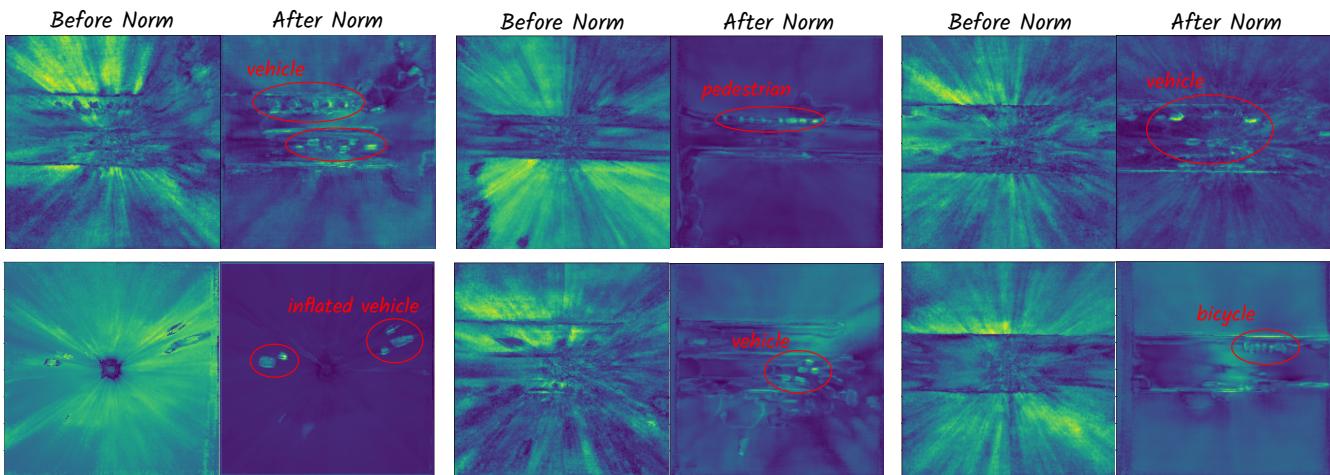
Figure 7: Visualization of BEV features before and after semantic-conditional normalization highlights the responses o BEV grids, particularly for instance objects. Consequently, it extracts discriminative BEV features for forecasting and planning.

Figure 8: Qualitative results of controllable generation, using the high-level steering angle or low-level velocity conditions.

the same ray in 3D space often correspond to the same pixel in the image, leading to the extraction of similar feature representations. Consequently, these ray-shaped features are not sufficiently discriminative for semantic occupancy predictions.

To address this issue, we propose semantic-conditional normalization, which emphasizes BEV features with higher semantic-conditional probabilities, making the BEV embeddings more semantically discriminative. As illustrated in the visualizations of BEV features After Normalization in Figure 7, this approach efficiently highlights the responses of BEV grids, particularly for instance objects such as vehicles, pedestrians, and bicycles, which are crucial for occupancy prediction and collision avoidance. Meanwhile, it preserves both semantic and geometric information, benefiting subsequent semantic occupancy forecasting and planning.

D.3 Semantic Loss

In Table 10, we ablate the effectiveness of various loss functions for semantic occupancy forecasting, including crossentropy loss, binary occupancy loss, and Lovasz loss. The ´ results reveal that using only cross-entropy loss achieves satisfactory performance while adding additional supervision leads to further gains. Interestingly, semantic losses also enhance the performance of flow forecasting on ${\mathrm{VPQ}}_f^{\ast }$ , demonstrating that accurate object center localization is crucial for instance association.

E Additional Visualizations

E.1 Action Controllability

In Figure 8, we present additional qualitative results of the controllable generation of Drive-OccWorld, which takes historical visual images and diverse action conditions as input to predict various future states. The results illustrate that Drive-OccWorld can generate plausible future occupancies based on specific ego actions. For instance, the bottom section showcases the generated occupancies using different ego velocities, where high velocity brings the ego vehicle dangerously close to colliding with pedestrians. These qualitative results demonstrate the potential of Drive-OccWorld as a neural simulator to generate realistic environmental states for autonomous driving, facilitating a broader range of downstream applications.

图7：语义条件归一化前后BEV 特征的可视化突出了鸟瞰网格的响应，特别是对实例对象的响应。因此，它为预测和规划提取了具有判别性的 BEV 特征。

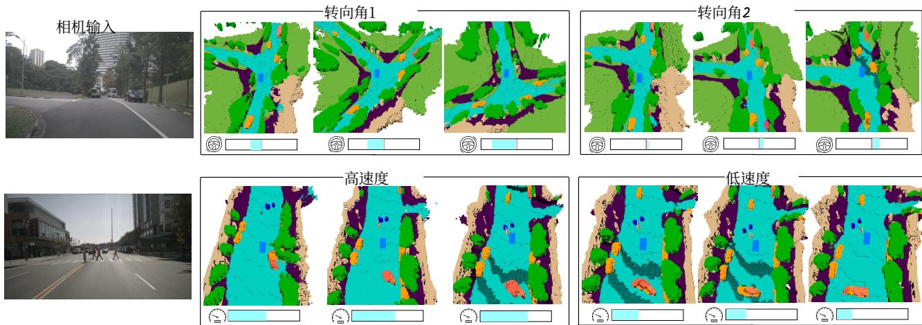
Figure 8: 可控生成的定性结果，使用高级的 转向角 或低级的 速度 条件。

三维空间中同一射线上的航点通常对应图像中的同一像素，导致提取出相似的特征表示。因此，这些射线状特征对于语义占据预测的区分度不足。

为了解决这个问题，我们提出了语义条件归一化，它强调具有更高语义条件概率的 BEV 特征，使 BEV嵌入在语义上更具判别性。如 归一化后 在图7 的BEV 特征可视化所示，该方法有效突出 BEV 网格的响应，特别是诸如车辆、行人和自行车等实例对象，这些对象对于占用预测和碰撞避免至关重要。同时，它保留了语义和几何信息，有利于后续的语义占用预测和规划。

D.3 语义损失

在表10中，我们对语义占用预测的各种损失函数的有效性进行了消融，包括交叉熵损失、二值占用损失和Lov´asz 损失。结果表明，仅使用交叉熵损失即可取得令人满意的表现

，而加入额外的监督则能带来进一步的提升。有趣的是，语义损失也提升了 ${\mathrm{VPQ}}_f^{\ast }$ 上流量预测的性能，这表明准确的物体中心定位对于实例关联至关重要。

E 额外可视化

E.1 动作可控性

在图8 中，我们展示了 Drive‑OccWorld 可控生成的更多定性结果，Drive‑OccWorld 以历史视觉图像和多样的动作条件作为输入来预测不同的未来状态。结果表明，Drive‑OccWorld 可以基于特定的自车动作生成合理的未来占用。例如，底部部分展示了使用不同自车速度生成的占用，高速度会使自车危险地接近与行人发生碰撞。这些定性结果展示了Drive‑OccWorld 作为神经模拟器生成逼真环境状态以支持自动驾驶的潜力，便于更广泛的下游应用。

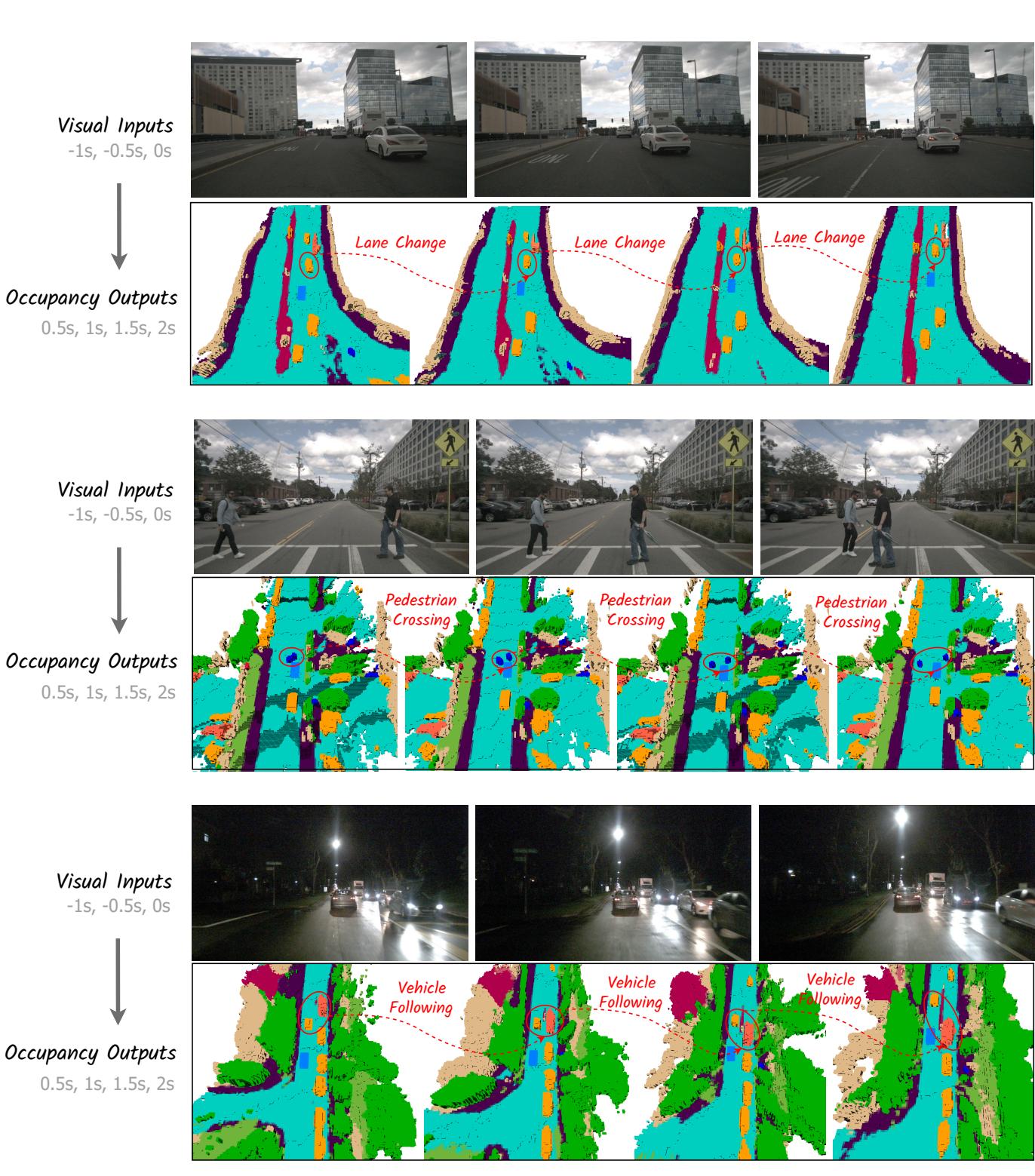
Figure 9: Qualitative results for vision-centric 4D occupancy forecasting on the nuScenes validation set. Top: historical visual inputs over three timestamps, showing only the front images for simplicity. Bottom: future occupancy predictions for two seconds. Notable movable objects are highlighted in red circles. The first section indicates a vehicle changing lanes, the second section shows two pedestrians crossing the road, and the third section depicts the ego vehicle following a preceding car.

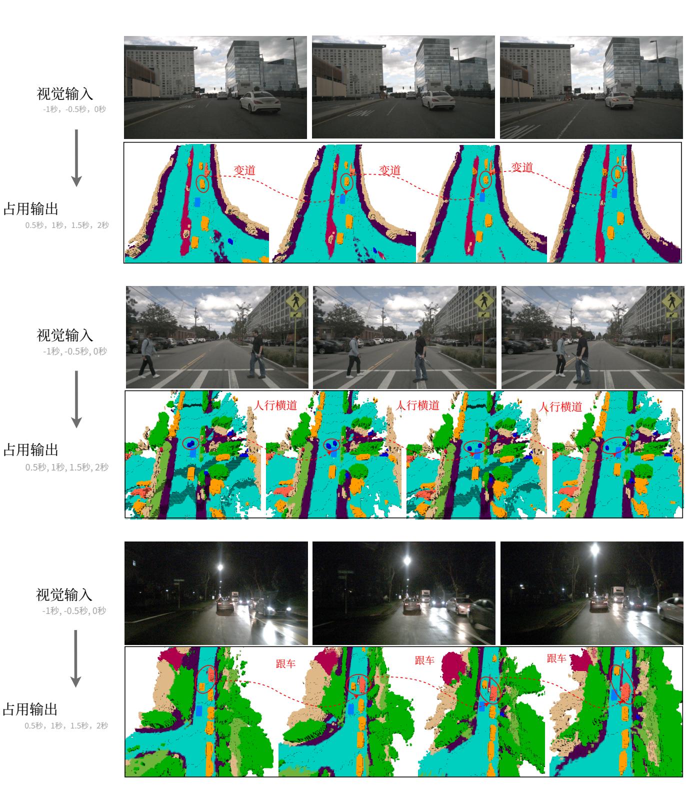
图9： 以视觉为中心的四维占用预测在 nuScenes 验证集上的定性结果。上：跨越三个时间戳的历史视觉输入，为简洁起见仅显示前向图像。下：两秒钟的未来占用预测。显著的可移动物体用 红色圆圈 标出。第一部分显示车辆变道，第二部分展示两名行人过马路，第三部分描绘自车跟随前车。

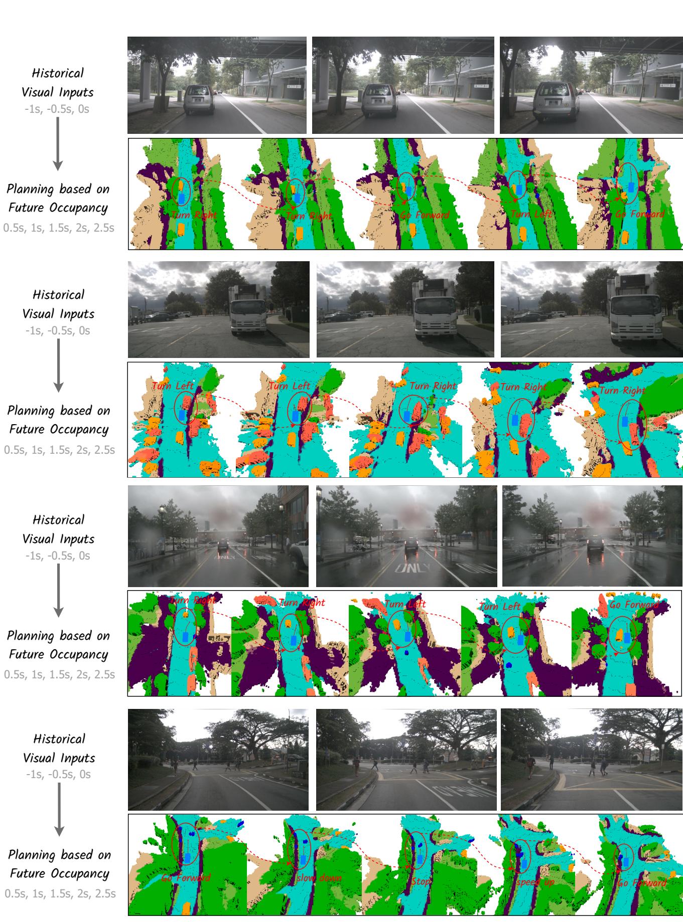
Figure 10: Qualitative results for continuous forecasting and planning on the nuScenes validation set. Top: historical visual inputs over three timestamps, showing only the front images for simplicity. Bottom: future occupancy and planning results for five timestamps, with predicted trajectories highlighted in red arrows. The first three sections show the ego vehicle avoiding preceding cars, while the last section illustrates the ego car slowing down and stopping until the pedestrians in front have passed.

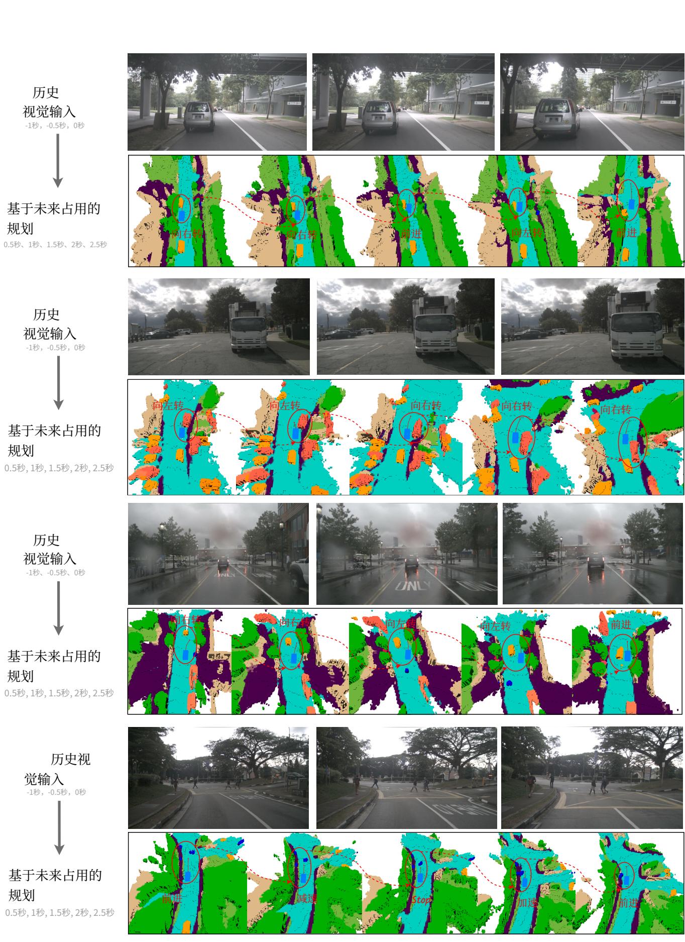
图10： 在nuScenes 验证集上进行连续预测与规划的定性结果。 上：三个时间戳的历史视觉输入，为简洁起见仅显示前向图像。下：五个时间戳的未来占用和规划结果，预测轨迹以 redarrows 高亮显示。前三个部分展示了自车避开前方车辆，最后一部分则展示自车减速并停止，直到前方行人通过。

E.2 4D Occupancy Forecasting

In Figure 9, we present additional qualitative results for vision-centric 4D occupancy forecasting. The historical visual inputs over three timestamps are displayed in the top part, while the future occupancy predictions for two seconds are shown in the bottom part. Notable movable objects around the ego vehicle are highlighted with red circles.

The first section depicts a vehicle changing its driving lane from right to left, with Drive-OccWorld accurately predicting its future states. The second section illustrates two pedestrians crossing the road in front of the ego vehicle, and Drive-OccWorld successfully predicts their future trajectories. The third section reveals that Drive-OccWorld learns that the ego vehicle follows a preceding car, even under nighttime conditions. These results demonstrate that DriveOccWorld understands how the world evolves by accurately modeling the dynamics of movable objects and the future states of the static environment.

E.3 Trajectory Planning

In Figure 10, we present qualitative results of trajectory planning based on occupancy predictions. The predicted trajectories are highlighted with red arrows.

The first three sections demonstrate how the ego vehicle avoids preceding cars by turning, showcasing the effectiveness of the agent-safety cost in preventing collisions. The third section also indicates that Drive-OccWorld is adaptable to rainy conditions. The last section illustrates the ego vehicle slowing down and stopping to allow pedestrians in front to cross the road before resuming speed for future navigation.

E.2 4D 占用预测

在图9中，我们展示了以视觉为中心的四维占用预测的额外定性结果。顶部显示了跨越三个时间戳的历史视觉输入，而底部显示了未来两秒的占用预测。围绕自车的显著可移动物体用红色圆圈标出。

第一部分展示了一辆车辆从右车道变换到左车道，Drive‑OccWorld 能准确预测其未来状态。第二部分展示了两名行人在自车前方过马路，Drive‑OccWorld 成功预测了他们的未来轨迹。第三部分表明即使在夜间条件下，Drive‑OccWorld 也学会了自车跟随前方车辆。这些结果表明，Drive‑OccWorld 通过准确建模可移动对象的动力学和静态环境的未来状态，理解了世界如何演变。

E.3 轨迹规划

在图10中，我们展示了基于占用预测的轨迹规划的定性结果。预测的轨迹以红色箭头标出。

前三个部分展示了自车如何通过转向规避前方车辆，体现了代理安全代价在防止碰撞方面的有效性。第三部分还表明 Drive‑OccWorld 能适应雨天条件。最后一部分展示了自车减速并停车以让前方行人过马路，然后恢复速度继续导航。

---

---

---

http://arxiv.org/abs/2408.14197