DrivingWorld: Constructing World Model for Autonomous Driving via Video GPT

Xiaotao $\mathrm{H}{\mathrm{u}}^{1,2}$ * Wei $\mathrm{Yi}{\mathrm{n}}^2\ast †$ Mingkai Jia1,2 Junyuan Deng1,2 Xiaoyang Guo2 Qian Zhang2 Xiaoxiao Long1 ‡ Ping Tan1

1 The Hong Kong University of Science and Technology 2 Horizon Robotics

https://tinyurl.com/DrivingWorld

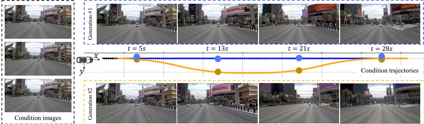
Figure 1. Controllable generation results of our method. Our method takes a short video clip as input and can generate multiple possible future driving scenarios conditioned on different pre-defined trajectory paths. We use one straightforward path and one curved path as examples, and the results show that our method achieves accurate control and future prediction.

Abstract

Recent successes in autoregressive (AR) generation models, such as the GPT series in natural language processing, have motivated efforts to replicate this success in visual tasks. Some works attempt to extend this approach to autonomous driving by building video-based world models capable of generating realistic future video sequences and predicting ego states. However, prior works tend to produce unsatisfactory results, as the classic GPT framework is designed to handle 1D contextual information, such as text, and lacks the inherent ability to model the spatial and temporal dynamics essential for video generation. In this paper, we present DrivingWorld, a GPT-style world model for autonomous driving, featuring several spatial-temporal fusion mechanisms. This design enables effective modeling of both spatial and temporal dynamics, facilitating high-fidelity, long-duration video generation. Specifically, we propose a next-state prediction strategy to model temporal coherence between consecutive frames and apply a next-token prediction strategy to capture spatial information within each frame. To further enhance generalization ability, we propose a novel masking strategy and reweighting strategy for token prediction to mitigate long-term drifting issues and enable precise control. Our work demonstrates the ability to produce high-fidelity and consistent video clips of over 40 seconds in duration, which is over 2 times longer than state-of-the-art driving world models. Experiments show that, in contrast to prior works, our method achieves superior visual quality and significantly more accurate controllable future video generation. Our code is available at https://github.com/YvanYin/DrivingWorld.

1. Introduction

In recent years, autoregressive (AR) learning schemes have achieved significant success in natural language processing, as demonstrated by models like the GPT series [3, 28, 29]. These models predict future text responses from past data, making AR approaches the leading candidates in the pursuit of Artificial General Intelligence (AGI). Inspired by these advancements, many researchers have sought to replicate

DrivingWorld：通过 Video GPT 构建用于自动驾驶的世界模型

Xiaotao Hu1,2 ${}^{\ast }$ Wei $\mathrm{Yi}{\mathrm{n}}^2{\ast }_{†}$ Mingkai Jia1,2 Junyuan Deng1,2 Xiaoyang Guo2 Qian Zhang2
Xiaoxiao Long1 ${}^{‡}$ Ping Tan11 香港科技大学2 Horizon Robotics

https://tinyurl.com/DrivingWorld

Figure 1. 我们方法的可控生成结果。我们的方法以短视频片段作为输入，并能够在不同预定义轨迹路径的条件下生成多种可能的未来驾驶场景。我们以一条直线路径和一条弯路线为示例，结果表明我们的方法在控制和未来预测上均能取得准确的表现。

摘要

最近在自回归（AR）生成模型方面的成功，例如自然语言处理领域的GPT系列，激发了将这种成功复制到视觉任务的尝试。一些工作试图通过构建基于视频的世界模型来扩展该方法，以实现生成逼真的未来视频序列并预测自车状态。然而，先前的工作往往产生不尽如人意的结果，因为经典的GPT框架是为处理一维上下文信息（如文本）而设计的，缺乏对视频生成所必需的时空动态的固有建模能力。在本文中，我们提出了DrivingWorld，这是一种用于自动驾驶的GPT风格世界模型，具有若干时空融合机制。该设计能够有效建模空间和时间动态，从而促进高保真、长时长的视频生成。具体来说，我们提出了一种下一状态预测策略来建模连续帧之间的时间一致性，并应用了一种下一令牌

预测策略以捕捉每一帧内的空间信息。为进一步增强泛化能力，我们提出了一种新颖的掩码策略和用于代币预测的重加权策略，以缓解长期漂移问题并实现精确控制。我们的工作展示了生成时长超过 40 秒的高保真且一致的视频片段的能力，长度是现有最先进驾驶世界模型的两倍以上。实验证明，与以往工作相比，我们的方法在视觉质量上更优，并且在可控的未来视频生成方面显著更准确。我们的代码可在以下位置获得

https://github.com/YvanYin/DrivingWorld。

1. 引言

近年来，自回归（AR）学习方案在自然语言处理领域取得了显著成功，正如 GPT 系列 [3, 28, 29] 等模型所展示的那样。这些模型根据过去的数据预测未来的文本响应，使得自回归方法成为追求通用人工智能（AGI）时的首选候选。受这些进展的启发，许多研究者试图复制

this success in visual tasks, such as building vision-based world models for autonomous driving [17].

A critical capability in autonomous driving systems is future event prediction [10]. However, many prediction models rely heavily on large volumes of labeled data, making them vulnerable to out-of-distribution and long-tail scenarios [27, 30, 37]. This is especially problematic for rare and extreme cases, such as accidents, where obtaining sufficient training data is challenging. A promising solution lies in autoregressive world models, which learn comprehensive information from unlabeled data like massive videos through unsupervised learning. This enables more robust decisionmaking in driving scenarios. These world models have the potential to reason under uncertainty and reduce catastrophic errors, thereby improving the generalization and safety of autonomous driving systems.

The prior work, GAIA-1 [17], is the first to extend the GPT framework from language to video, aiming to develop a video-based world model. Similar to natural language processing, GAIA transforms 4D temporally correlated frames into a sequence of 1D feature tokens and employs the nexttoken prediction strategy to generate future video clips. However, the classic GPT framework, primarily designed for handling 1D contextual information, lacks the inherent capability to effectively model the spatial and temporal dynamics necessary for video generation. As a result, videos produced by GAIA-1 often suffer from low quality and noticeable artifacts, highlighting the challenge of achieving fidelity and coherence within a GPT-style video generation framework.

In this paper, we introduce DrivingWorld, a driving world model built on a GPT-style video generation framework. Our primary goal is to enhance the modeling of temporal coherence in an autoregressive framework to create more accurate and reliable world models. To achieve this, our model incorporates three key innovations: 1) Temporal-Aware Tokenization: We propose a temporal-aware tokenizer that transforms video frames into temporally coherent tokens, reformulating the task of future video prediction as predicting future tokens in the sequence. 2) Hybrid Token Prediction: Instead of relying solely on the next-token prediction strategy, we introduce a next-state prediction strategy to better model temporal coherence between consecutive states. Afterward, the next-token prediction strategy is applied to capture spatial information within each state. 3) Long-time Controllable Strategies: To improve robustness, we implement random token dropout and balanced attention strategies during autoregressive training, enabling the generation of longer-duration videos with more precise control.

Overall, our work enhances temporal coherence in video generation using the AR framework, learning meaningful representations of future evolution. Experiments show that the proposed model achieves good generalization performance, is capable of generating over 40 seconds video sequences, and provides accurate next-step trajectory predictions, maintaining a reasonable level of controllability.

2. Related Work

World Model. The world model [24] captures a comprehensive representation of the environment and forecasts future states based on a sequence of actions. World models have been extensively explored in both game [11–13] and laboratory environments [40]. Dreamer [11] trained a latent dynamics model using past experiences to forecast state values and actions within a latent space. DreamerV2 [12] built upon the original Dreamer model, reaching human-level performance in Atari games. DreamerV3 [13] employed larger networks and successfully learned to acquire diamonds in Minecraft from scratch. DayDreamer [40] extended Dreamer [11] to train four robots in the real world, successfully tackling locomotion and manipulation tasks.

Recently, world models for driving scenarios have garnered significant attention in both academia and industry. Most previous works [1, 6, 7, 15] have been limited to simulators or well-controlled lab environments. Drive-WM [39] explored real-world driving planners using diffusion models. GAIA-1 [17] investigated real-world driving planners based on autoregressive models, but GAIA-1 had large parameters and computational demands, which increased as the number of condition frames grew. In this paper, we propose an efficient world model in an autoregressive framework for autonomous driving scenarios.

VQVAE. VQVAE [36] learned a discrete codebook representation via vector quantization to model image distributions. VQGAN [8] improved realism by incorporating LPIPS loss [46] and adversarial PatchGAN loss [18]. MoVQ [47] tackled VQGAN’s spatially conditional normalization issue by embedding spatially variant information into quantized vectors. LlamaGen [33] further fine-tuned VQGAN, showing that a smaller codebook vector dimension and a larger codebook size could enhance reconstruction performance. While VQGAN-based structures were widely used, some methods explored more efficient architectures. ViTVQGAN [43] replaced the convolutional encoder-decoder with a vision transformer, improving the model’s ability to capture long-range dependencies. VAR [34] employed a multi-scale structure to predict subsequent scales from previous ones, enhancing generation quality and speed. However, these methods focused on single-image processing, preventing them from capturing temporal consistency. To address this, we propose a temporal-aware tokenizer and decoder.

Video Generation. Currently, there are three mainstream video generation models: GAN-based, diffusion-based, and GPT-based methods. GAN-based methods [31, 35, 44] often face several challenges, such as mode collapse, where the diversity of the videos generated by the generator becomes limited. Additionally, the adversarial learning between the 在视觉任务中的这一成功，例如为自动驾驶构建基于视 觉的世界模型 [17]。

自动驾驶系统中的一项关键能力是未来事件预测[10]。然而，许多预测模型在很大程度上依赖大量有标签数据，使其在分布外和长尾场景下脆弱 [27, 30, 37]。这对于诸如事故等罕见且极端的情况尤为成问题，因为获取足够的训练数据具有挑战性。一种有前景的解决方案是自回归世界模型，它们通过无监督学习从大量视频等无标签数据中学习全面信息，从而在驾驶场景中实现更鲁棒的决策。这些世界模型有可能在不确定性下进行推理并减少灾难性错误，从而提升自动驾驶系统的泛化能力和安全性。

先前的工作 GAIA‑1 [17], 是首个将 GPT 框架从语言扩展到视频、旨在开发基于视频的世界模型的工作。类似于自然语言处理，GAIA 将四维时序相关帧转换为一维特征标记序列，并采用下一个标记预测策略来生成未来的视频片段。然而，经典的 GPT 框架主要为处理一维上下文信息而设计，缺乏有效建模视频生成所需时空动态的内在能力。因此，GAIA‑1 生成的视频常表现出低质量和明显伪影，凸显了在 GPT 风格视频生成框架中实现真实感和连贯性所面临的挑战。

在本文中，我们介绍了DrivingWorld，一个基于GPT风格视频生成框架的驾驶世界模型。我们的主要目标是在自回归框架中增强时间一致性的建模，以创建更精确且更可靠的世界模型。为此，我们的模型引入了三项关键创新：1)Temporal-AwareTokenization：我们提出了一种时序感知标记器（temporal‑aware tokenizer），将视频帧转换为时间一致性的标记，将未来视频预测任务重新表述为序列中未来标记的预测。2) Hybrid Token Prediction：我们引入了混合标记预测策略，不再仅依赖下一个标记（next‑token）预测策略，而是先采用下一状态预测（next‑state prediction）策略以更好地建模相邻状态之间的时间一致性，随后再使用下一个标记预测策略来捕捉每个状态内的空间信息。3) Long-timeControllable Strategies：为了提高鲁棒性，我们在自回归训练中实施了随机标记丢弃（random token dropout）和balanced attention策略，从而能够生成更长时长且可控性更高的精确视频。

总体而言，我们的工作在自回归框架中增强了视频生成的时间一致性，学习到了对未来演变有意义的表示。实验表明，所提出的模型具有良好的泛化能力，能够生成超过40秒的视频序列，

并提供准确的下一步轨迹预测，同时保持合理的可控性。

2. 相关工作

世界模型。世界模型 [24]捕捉对环境的全面表示，并基于一系列动作预测未来状态。世界模型在游戏 [11–13]和实验室环境 [40]中都得到了广泛探索。Dreamer[11]使用过去的经验训练了一个潜在动力学模型，以在潜在空间中预测状态值和动作。DreamerV2[12]在原始Dreamer 模型的基础上改进，在 Atari 游戏 中达到了人类水平的表现。DreamerV3 [13] 采用了更大的网络，并成功从零开始学会在 Minecraft 中获取钻石。DayDreamer [40] 将 Dreamer [11] 扩展到在真实世界中训练四台机器人，成功应对了运动控制和操控任务。

近来，用于驾驶场景的世界模型在学术界和产业界都引起了广泛关注。大多数以往工作 [1,6,7,15]仅限于模拟器或受控良好的实验室环境。Drive‑WM[39]使用扩散模型探索了真实世界的驾驶规划器。GAIA‑1[17]基于自回归模型研究了真实世界的驾驶规划器，但 GAIA‑1 拥有庞大的参数量和较高的计算需求，且随着条件帧数量的增加而增加。在本文中，我们提出了一种在自回归框架下用于自动驾驶场景的高效世界模型。

VQVAE。VQVAE [36] 通过向量量化学习到离散码本表示来建模图像分布。VQGAN [8]通过引入 LPIPS损失 [46] 和对抗 PatchGAN 损失 [18]提升了真实感。MoVQ [47]通过将空间可变信息嵌入量化向量来解决VQGAN 的空间条件归一化问题。LlamaGen [33]进一步微调了 VQGAN，表明较小的码本向量维度和较大的码本大小可以增强重建性能。尽管基于 VQGAN的结构被广泛使用，但一些方法探索了更高效的架构。ViT‑VQGAN [43] 用视觉变换器替换了卷积编码器‑解码器，提高了模型捕捉远程依赖的能力。VAR [34] 采用多尺度结构，从先前尺度预测后续尺度，从而提升了生成质量和速度。然而，这些方法侧重于单幅图像处理，无法捕捉时间一致性。为了解决这一问题，我们提出了一种时间感知分词器和解码器。

视频生成。目前，主流的视频生成模型有三类：基于GAN 的方法、基于扩散的方法和基于GPT的方法。基于 GAN 的方法 [31,35,44]通常面临若干挑战，例如模式崩溃，即生成器生成的视频多样性变得有限。此外，判别器与

generator and discriminator can lead to instability during training. One major issue with diffusion-based methods is their inability to generate precisely controlled videos. The stochastic nature of the diffusion process introduces randomness at each step, making it difficult to enforce strict control over specific attributes in the generated content. On the other hand, traditional GPT-based methods [14, 41] allow for a certain level of control, but their computational cost grows quadratically with the sequence length, significantly impacting model efficiency. In this paper, we propose a decoupled spatio-temporal world model framework, which ensures precise control while significantly reducing computational cost and improving model efficiency.

3. Method

Our proposed world model, DrivingWorld, leverages a GPTstyle architecture to predict future states with high efficiency, capable of extending predictions beyond 40 seconds at $10\mathrm{Hz}$ . This model is designed to comprehend past real-world states and forecast future video content and vehicle motions. DrivingWorld is specifically focused on predicting the next state at time $T+1$ based on the historical states from time 1 to $T$ , and we can generate long videos by sequentially predicting future states one by one. Each state at time $t$ is represented as $[{\theta }_t,(x_t,y_t),{\mathbf{I}}_t]$ , where ${\theta }_t$ is the vehicle’s orientation, $(x_t,y_t)$ is its location, and ${\mathbf{I}}_t$ is the current front-view image.

As shown in Figure 2, our proposed DrivingWorld not only generates future states $[{\theta }_{T+1},(x_{T+1},y_{T+1}),{\mathbf{I}}_{T+1}]$ based on past observations {[θt,(xt,yt),It]}t=1T\left\{ [ \theta _ { t } , ( x _ { t } , y _ { t } ) , \mathbf { I } _ { t } ] \right\} _ { t = 1 } ^ { T }{[θt​,(xt​,yt​),It​]}t=1T​ , but also supports controllable simulation of complex driving scenarios by manipulating the vehicle’s location and orientation. Section 3.1 details our proposed tokenizers for encoding temporal multimodal information into the unified latent space. To model the relationships between long-term sequential states, we introduce a GPT-style temporal multimodel decoupled world model in Section 3.2. To extract the state from the tokens predicted by the world model, we also introduce a temporal decoder, which is discussed in detail in Section 3.3. Additionally, we introduce long-term controllable strategies in Section 3.4 to address the drifting problem and enhance the robustness of the proposed world model.

3.1. Tokenizer

Tokenization [36, 47] converts continuous data into discrete tokens, enabling integration with language models and enhanced multimodal sequence modeling. In our approach, the tokenizer maps multimodal states into a unified discrete space, which enables accurate and controllable multimodal generation. To produce temporally consistent embeddings for images, we propose a temporal-aware vector quantized tokenizer. Our proposed vehicle pose tokenizer discretizes pose trajectories and integrates them into our DrivingWorld.

Prelimilary: Single Image Vector Quantized Tokenizer. The single image vector quantized (VQ) tokenizer, as described in [36], is designed to convert an image feature map $\mathbf{f}\in {\mathbb{R}}^{H\times W\times C}$ to discrete tokens $\mathbf{q}\in [K{]}^{H\times W}$ . The quantizer utilizes a learned discrete codebook $\mathcal{Z}\in {\mathbb{R}}^{K\times C}$ , containing $K$ vectors, to map each feature ${\mathbf{f}}^{(i,j)}$ to the index ${\mathbf{q}}^{(i,j)}$ of the closest code in $\mathcal{Z}$ . This method enables the conversion of continuous image data into discrete tokens.

Temporal-aware Vector Quantized Tokenizer. Singleimage VQ tokenizers often struggle to produce temporally consistent embeddings, causing discontinuous video predictions and hindering the training of the world model. The image sequence {It}t=1T\{ \mathbf { I } _ { t } \} _ { t = 1 } ^ { T }{It​}t=1T​ is encoded as {ft}t=1T\{ \mathbf { f } _ { t } \} _ { t = 1 } ^ { T }{ft​}t=1T​ , where each feature is processed independently, lacking temporal information.

To address this issue, we propose a temporal-aware vector quantized tokenizer designed to ensure consistent embeddings over time. Specifically, to capture temporal dependencies, we insert a self-attention layer both before and after VQGAN [8] quantization, where the attention operates along the temporal dimension. This allows our model to capture long-term temporal relationships between frames, improving coherence and consistency in the generated sequences. Our model builds upon the open-source VQGAN [8] implementation from LlammaGen [33]. The integration of our straightforward yet effective temporal self-attentions can be seamlessly incorporated into the original framework, followed by fine-tuning to develop a robust and generalizable temporal-aware VQ tokenizer. {ft}t=1T\{ \mathbf { f } _ { t } \} _ { t = 1 } ^ { T }{ft​}t=1T​ are fed into temporal self-attention $\mathcal{H}(\cdot )$ before performing quantization:

$${\mathbf{q}}_t^{(i,j)}=\underset{k\in [K]}{\mathrm{argmin}}{\Vert \log \mathrm{kup}(\mathcal{Z},k)-\mathcal{H}({\mathbf{f}}_1^{(i,j)},...,{\mathbf{f}}_T^{(i,j)})[t]\Vert }_2$$

where $\mathrm{lookup}(\mathcal{Z},k)$ denotes the $k$ -th vector in codebook $\mathcal{Z}$ . Vehicle Pose Tokenizer. To accurately represent the vehicle’s ego status, including its orientation $\theta$ and location $(x,y)$ , we adopt a coordinate system centered at the ego vehicle, as depicted in Figure 2. Instead of global poses, we adopt the relative poses between adjacent time steps. This is because global poses present a significant challenge due to the increasing magnitude of absolute pose values over longterm sequences. This growth makes normalization difficult and reduces model robustness. As sequences grow longer, managing these large pose values becomes increasingly difficult, hindering effective long-term video generation.

For the sequence of the vehicle’s orientation {θt}t=1T\left\{ \boldsymbol { \theta } _ { t } \right\} _ { t = 1 } ^ { T }{θt​}t=1T​ and location {(xt,yt)}t=1T\left\{ \left( x _ { t } , y _ { t } \right) \right\} _ { t = 1 } ^ { T }{(xt​,yt​)}t=1T​ , we propose to compute relative values for each time step with respect to the previous one. The relative location and orientation at the first time step is initialized as zero. The ego-centric status sequence is given by {Δθt}t=1T\left\{ \Delta \theta _ { t } \right\} _ { t = 1 } ^ { T }{Δθt​}t=1T​ and $\{(\Delta \overline{x_t},\Delta y_t){\}}_{t=1}^T$ . To tokenize them, we discretize the ego’s surrounding space. Specifically, we discretize the orientation into $\alpha$ categories, and the $X$ and $Y$ 生成器之间的对抗学习可能导致训练过程不稳定。基 于扩散的方法的一个主要问题是它们无法生成精确可 控的视频。扩散过程的随机性在每一步都会引入随机 性，使得难以对生成内容的特定属性施加严格控制。 另一方面，传统的基于GPT的方法 [14, 41] 允许在一 定程度上进行控制，但其计算开销随序列长度呈二次 增长，显著影响模型效率。本文提出了一种解耦时空 世界模型框架，既能确保精确控制，又能显著降低计 算成本并提高模型效率。

3. 方法

我们提出的世界模型，DrivingWorld，采用类似 GPT的架构以高效预测未来状态，能够以10Hz扩展预测超过40秒。该模型旨在理解过去的真实世界状态并预测未来的视频内容与车辆运动。Driv-ingWorld 专注于基于时间1到 $T$ 的历史状态预测时间 $T+1$ 的下一个状态，我们可以通过逐一顺序预测未来状态来生成长视频。每个时间 $t$ 的状态表示为 $\cdot {\theta }_t,(x_t,y_t),{\mathbf{I}}_t],$ ，其中 ${\theta }_t$ 是车辆的朝向， $(x_t,y_t)$ 是其位置，且 ${\mathbf{I}}_t$ 是当前的前视图像。

如图2所示，DrivingWorld 不仅生成未来状态$[{\theta }_{T+1},(x_{T+1},y_{T+1})$ ， ${\mathbf{I}}_{T+1}$ ]基于过去的观测{[θt,(xt,yt),It]}t=1T\left\{ \left[ \theta _ { t } , ( x _ { t } , y _ { t } ) , \mathbf { I } _ { t } \right] \right\} _ { t = 1 } ^ { T }{[θt​,(xt​,yt​),It​]}t=1T​ ，还通过操控车辆的位置和朝向支持复杂驾驶场景的可控仿真。第3.1节详细介绍我们提出的标记器，用于将时序多模态信息编码到统一潜在空间。为建模长期序列状态之间的关系，我们在第3.2节引入了一个类 GPT 的时序多模态解耦世界模型。为从世界模型预测的标记中提取状态，我们还在第3.3节讨论了一个时序解码器。此外，我们在第3.4 节引入了长期可控策略，以解决漂移问题并增强所提世界模型的鲁棒性。

3.1. Tokenizer

分词化 [36,47]将连续数据转换为离散令牌，从而实现与语言模型的集成并增强多模态序列建模。在我们的方法中，标记器将多模态状态映射到统一的离散空间，从而实现精确且可控的多模态生成。为了为图像生成时间一致的嵌入，我们提出了一种时序感知向量量化分词器。我们提出的车辆位姿分词器对位姿轨迹进行离散化，并将其集成到我们的 DrivingWorld 中。

Prelimilary: SingleImage Vector QuantizedTokenizer.单图像向量量化（VQ）分词器，正如在 [36],中所描述的，旨在将图像特征图f $\in {\mathbb{R}}^{H\times W\times C}$ 转换为离散标记$\mathbf{q}\in [K{]}^{H\times W}$ 。该量化器利用一个学习的离散码本$\mathcal{Z}\in {\mathbb{R}}^{K\times C}$ ，包含 $K$ 个向量，将每个特征 ${\mathbf{f}}^{(i,j)}$ 映射为与$\mathcal{Z}$ 中最接近代码的索 $|{\mathbf{q}}^{(i,j)}$ 。此方法使得连续的图像数据能够被转换为离散标记。

时序感知向量量化分词器。 单帧图像的 VQ 分词器通常难以产生时间上连贯的嵌入，导致视频预测出现不连续并阻碍世界模型的训练。图像序列 {It}t=1T\{ \mathbf { I } _ { t } \} _ { t = 1 } ^ { T }{It​}t=1T​ 被编码为 {ft}t=1T\{ \mathbf { f } _ { t } \} _ { t = 1 } ^ { T }{ft​}t=1T​ ，其中每个特征独立处理，缺乏时间信息。

为了解决这一问题，我们提出了一种时序感知的向量量化分词器，旨在确保随时间保持一致的嵌入。具体来说，为了捕捉时间依赖性，我们在 VQGAN [8]量化的之前和之后各插入一层自注意力层，注意力沿时间维度作用。这样我们的模型能够捕捉帧与帧之间的长期时序关系，从而提高生成序列的连贯性和一致性。我们的模型基于 LlammaGen [33]开源的VQGAN [8] 实现构建。将我们这种简单但有效的时序自注意力无缝集成到原始框架中，并通过微调，可得到稳健且具广泛适用性的时序感知 VQ 分词器。

{ft}t=1T\{ \mathbf { f } _ { t } \} _ { t = 1 } ^ { T }{ft​}t=1T​ 在量化前被送入时序自注意力 $\mathcal{H}$ （·）：

$${\mathbf{q}}_t^{(i,j)}=\underset{k\in [K]}{\mathrm{argmin}}{\Vert \log \mathrm{kup}(\mathcal{Z},k)-\mathcal{H}({\mathbf{f}}_1^{(i,j)},...,{\mathbf{f}}_T^{(i,j)})[t]\Vert }_2$$

其中 $\mathrm{lookup}(\mathcal{Z},k)$ 表示码本中的第 $k$ 个向量 ${\mathcal{Z}}_{\circ }$ 。车辆位姿分词器。 为了准确表示车辆自身状态，包括其朝向 $\theta$ 和位置 $(x,y)$ ，我们采用以自车为中心的坐标系，如图 2所示。我们不使用全局位姿，而是采用相邻时间步之间的相对位姿。这是因为全局位姿在长期序列中绝对位姿值会不断增大，带来显著挑战：该增长使得归一化变得困难并降低模型的鲁棒性。随着序列变长，处理这些大幅位姿值变得愈发困难，从而妨碍有效的长期视频生成。

对于车辆朝向序列 {θt}t=1T\left\{ \boldsymbol { \theta } _ { t } \right\} _ { t = 1 } ^ { T }{θt​}t=1T​ 和位置 {(xt,yt)}t=1T,\left\{ \left( x _ { t } , y _ { t } \right) \right\} _ { t = 1 } ^ { T } ,{(xt​,yt​)}t=1T​, ，我们提出对每个时间步相对于前一时刻计算相对值。第一个时间步的相对位置和朝向初始化为零。自车中心状态序列由 {Δθt}t=1T\left\{ \Delta \theta _ { t } \right\} _ { t = 1 } ^ { T }{Δθt​}t=1T​ 和 {(Δxt,Δyt)}t=1T\left\{ ( \Delta x _ { t } , \Delta y _ { t } ) \right\} _ { t = 1 } ^ { T }{(Δxt​,Δyt​)}t=1T​ 给出。为将其分词，我们对自车周围空间进行离散化。具体地，我们将朝向离散为 $\alpha$ 类别，而 $X$ 和 $Y$

Figure 2. Pipeline of DrivingWorld. The vehicle orientations {θt}t=1T\{ \theta _ { t } \} _ { t = 1 } ^ { T }{θt​}t=1T​ , ego locations $\{(x_t,y_t){\}}_{t=1}^T$ , and a front-view image sequence {Itˉ}t=1T\{ \bar { \mathbf { I } _ { t } } \} _ { t = 1 } ^ { T }{It​ˉ​}t=1T​ are taken as the conditional input, which are first tokenized as latent embeddings. Then our proposed multi-modal world model attempts to comprehend them and forecast the future states, which are detokenized to the vehicle orientation ${\hat{\theta }}_{T+1}$ , location $\left({\hat{x}}_{T+1},{\hat{y}}_{T+1}\right)$ , and the front-view image ${\hat{\mathbf{I}}}_{T+1}$ . With the autoregressive process, we can generate over 40 seconds videos.

axes into $\beta$ and $\gamma$ bins, respectively. Thus, the relative pose at time $t$ is tokenized as follows:

$$\begin{array}{l}{\varphi }_t=\lfloor \frac{\Delta {\theta }_t-{\theta }_{min}}{{\theta }_{max}-{\theta }_{min}}\alpha \rfloor ,\\ v_t=\lfloor \frac{\Delta x_t-x_{min}}{x_{max}-x_{min}}\beta \rfloor \cdot \gamma +\lfloor \frac{\Delta y_t-y_{min}}{y_{max}-y_{min}}\gamma \rfloor .\end{array}$$

Finally, we process the past $T$ real-world states $\{[{\theta }_t,({\stackrel{\cdot }{x}}_t,y_t),{\mathbf{I}}_t]{\}}_{t=1}^T$ and tokenize them into a discrete sequence {[ϕt,vt,qt]}t=1T\left\{ \left[ \phi _ { t } , v _ { t } , \mathbf { q } _ { t } \right] \right\} _ { t = 1 } ^ { T }{[ϕt​,vt​,qt​]}t=1T​ , where each token is a discrete representation of the vehicle’s state at each time step.

3.2. World Model

The world model aims to comprehend past state inputs, mimic real-world dynamics, and predict future states. In our context, it forecasts upcoming driving scenarios and plans a feasible future trajectory. To do this, the world model concatenates historical state tokens {[ϕt,v˙t,qt]}t=1T\left\{ \left[ \phi _ { t } , \dot { v } _ { t } , \mathbf { q } _ { t } \right] \right\} _ { t = 1 } ^ { T }{[ϕt​,v˙t​,qt​]}t=1T​ into a long sequence, where the 2D image tokens are unfolded into a 1D form in zig-zag order. Thus the objective is to predict the next state rT +1 = (ϕT +1, vT +1, q1T +1, . . . , qH×WT +1 based on the sequence of past observations {rt}Tt=1, capturing both temporal and multimodal dependencies. Note that all discrete tokens from different modalities are mapped into a shared latent space by their respective learnable embedding layers before being fed to the world model, i.e. ${\mathbf{h}}_t=Emb({\mathbf{r}}_t)$ . All subsequent processes are conducted within this latent space.

Prelimilary: Next-Token Prediction. A straightforward method is to use the GPT-2 [29] structure for 1D sequential next-token prediction. Figure 3 (a) shows a simplified example. The causal attention is applied for next-token prediction and the $i$ -th token in $T+1$ is modeled as:

$${\hat{\mathbf{r}}}_{T+1}^i=\mathcal{G}([sos],{\mathbf{r}}_1,\dots ,{\mathbf{r}}_T,{\hat{\mathbf{r}}}_{T+1}^1,\dots ,{\hat{\mathbf{r}}}_{T+1}^{i-1}),$$

where [sos] denotes the start-of-sequence token, $\mathbf{r}$ is the ground truth tokens, $\hat{\mathbf{r}}$ is the predict tokens, and $\mathcal{G}$ represent

GPT-2 [29] model. However, such a 1D design is inadequate for our specific scenarios. Predicting long-term videos requires generating tens of thousands of tokens, which is significantly time-consuming. Additionally, it overlooks the spatially structured image features inherent in images.

Therefore, we propose a next-state prediction pipeline, which consists of two modules: one integrates temporal and multimodal information for next-state feature generation (i.e. Temporal-multimodal Fusion Module), and the other is an autoregressive module (i.e. Internal-state Autoregressive Module) for high-quality internal-state token generation.

Temporal-multimodal Fusion Module. Our temporalmultimodal module is composed of a separate temporal layer and a multimodal layer. This decouples the processing of temporal and multimodal information, thereby improving both training and inference speed while also reducing GPU memory consumption. As shown in Figure 3 (b), we propose to employ a causal attention mask in the temporal transformer layer ${\mathcal{F}}_a(\cdot )$ , where each token only attends to itself and tokens at the same sequential position from all previous frames, fully leveraging temporal information.

$${\tilde{\mathbf{h}}}_t^i={\mathcal{F}}_a({\mathbf{h}}_1^i,\dots ,{\mathbf{h}}_t^i),i\in [1,H\times W+2],t\in [1,T].$$

In the multimodal information fusion layer ${\mathcal{F}}_b(\cdot )$ , we employ a bidirectional mask in the same frame, which is designed to fully integrate internal-state multimodal information and facilitates interactions between modalities. Each token attends to other tokens from the same time step,

$${\mathring{\mathbf{h}}}_t={\mathcal{F}}_b({\tilde{\mathbf{h}}}_t),t\in [1,T].$$

The temporal and multimodal layers are alternately stacked for $N$ layers to form this module.

Internal-state Autoregressive Module. After the temporalmultimodal module, we obtain features for future frame state prediction. A naive approach is to predict nextstate tokens $h_t$ at the same time. Recently, multiple 轴分别离散为 $\beta$ 和 $\gamma$ 个区间。因此，时刻 $t$ 的相对位姿被如 下分词：

图 $2_{\circ }$ 。Pipeline of DrivingWorld。车辆朝向 {θt}t=1T\{ \boldsymbol { \theta } _ { t } \} _ { t = 1 } ^ { T }{θt​}t=1T​ 、自车位置 $\{(x_t,y_t){\}}_{t=1}^T$ 和前视图像序列 {It}t=1T\{ \mathbf { I } _ { t } \} _ { t = 1 } ^ { T }{It​}t=1T​ 被作为条件输入，首先被标记化为潜在嵌入。然后我们提出的多模态世界模型 ˆ 试图理解它们并预测未来状态，这些预测被去标记化为车辆朝向 ${\theta }_{T+1\mathrm{s}}$ 、位置 $\left({\hat{x}}_{T+1},{\hat{y}}_{T+1}\right)$ 和前视图像 ${\hat{\mathbf{I}}}_{T+1\circ }$ 。通过自回归过程，我们可以生成超过 40 秒的视频。

$$\begin{array}{l}{\varphi }_t=\lfloor \frac{\Delta {\theta }_t-{\theta }_{min}}{{\theta }_{max}-{\theta }_{min}}\alpha \rfloor ,\\ v_t=\lfloor \frac{\Delta x_t-x_{min}}{x_{max}-x_{min}}\beta \rfloor \cdot \gamma +\lfloor \frac{\Delta y_t-y_{min}}{y_{max}-y_{min}}\gamma \rfloor .\end{array}$$

最后，我们处理过去 $T$ 真实世界状态 {[θt,(xt,yt),It]}t=1T\left\{ \left[ \theta _ { t } , ( x _ { t } , y _ { t } ) , \mathbf { I } _ { t } \right] \right\} _ { t = 1 } ^ { T }{[θt​,(xt​,yt​),It​]}t=1T​ 并将它们标记化为一个离散序列 {[ϕt,vt,qt]}t=1T\left\{ \left[ \phi _ { t } , v _ { t } , \mathbf { q } _ { t } \right] \right\} _ { t = 1 } ^ { T }{[ϕt​,vt​,qt​]}t=1T​ ，其中每个代币都是每个时间步车辆状态的离散表示。

3.2. 世界模型

世界模型旨在理解过去的状态输入、模拟真实世界的动力学并预测未来状态。在我们的语境中，它负责预判即将到来的驾驶场景并规划可行的未来轨迹。为此，世界模型将历史状态令牌 {[ϕt,vt,qt]}t=1T\left\{ \left[ \phi _ { t } , v _ { t } , \mathbf { q } _ { t } \right] \right\} _ { t = 1 } ^ { T }{[ϕt​,vt​,qt​]}t=1T​ 串联成一长序列，其中二维图像令牌以之字形顺序展开为一维形式。因此，其目标是基于过去观测的序列 {rt}t=1T\left\{ { \bf r } _ { t } \right\} _ { t = 1 } ^ { T }{rt​}t=1T​ 预测下一个状态 ${\mathbf{r}}_{T+1}=({\varphi }_{T+1},v_{T+1},{\mathbf{q}}_{T+1}^1,\dots ,{\mathbf{q}}_{T+1}^{H\times W});$ ，同时捕捉时序和多模态依赖。注意，来自不同模态的所有离散令牌在被送入世界模型之前，先由各自可学习的嵌入层映射到共享潜在空间，即 ${\mathbf{h}}_t=Emb({\mathbf{r}}_t{)}_{\circ }$ 此后所有过程均在该潜在空间中进行。

预备知识：下一个标记预测。一种直接的方法是将GPT‑2[29]结构用于一维序列的一维序列下一个标记预测。图3(a) 显示了一个简化示例。因果注意力用于下一个标记预测，且 $i\cdot$ ‑th 代币在 $T+1$ 中被建模为：

${\hat{\mathbf{r}}}_{T+1}^i=\mathcal{G}([sos],{\mathbf{r}}_1,\dots ,{\mathbf{r}}_T,{\hat{\mathbf{r}}}_{T+1}^1,\dots ,{\hat{\mathbf{r}}}_{T+1}^{i-1}),$ (3)where $[sos]$ 表示序列起始代币， $\mathbf{r}$ 是 真实标记， $\hat{\mathbf{r}}$ 是预测标记，且 $\mathcal{G}$ 表示

GPT‑2 [29] 模型。然而，这样的一维设计对于我们的特定场景是不足的。预测长期视频需要生成数万标记，这在时间上非常耗费。此外，它也忽视了图像固有的具有空间结构的图像特征。

因此，我们提出了一个下一状态预测流水线，该流水线由两个模块组成：一个用于整合时间和多模态信息以生成下一状态特征（即时序多模态融合模块），另一个是用于高质量内部状态代币生成的自回归模块（即内部状态自回归模块）。

时序多模态融合模块。我们的时序多模态模块由独立的时序层和多模态层组成。这将时序信息和多模态信息的处理解耦，从而提高训练与推理速度，同时也降低 GPU 内存消耗。如图3(b) 所示，我们建议在时序transformer 层中采用因果注意力掩码 ${\mathcal{F}}_a(\cdot )$ ，在该掩码下，每个代币仅关注其自身以及来自所有先前帧的相同序列位置的代币，从而充分利用时序信息。

$${\tilde{\mathbf{h}}}_t^i={\mathcal{F}}_a({\mathbf{h}}_1^i,\dots ,{\mathbf{h}}_t^i),i\in [1,H\times W+2],t\in [1,T].$$

在多模态信息融合层 ${\mathcal{F}}_b(\cdot )$ 中，我们在同一帧内采用了双向掩码，旨在充分整合内部状态多模态信息并促进模态间的交互。每个标记会关注同一时间步的其他标记，

$${\mathring{\mathbf{h}}}_t={\mathcal{F}}_b({\tilde{\mathbf{h}}}_t),t\in [1,T].$$

时间和多模态层交替堆叠，共 $N$ 层以构成该模块。

内部状态自回归模块。 在时序多模态模块之后，我们获得用于未来帧状态预测的特征。一种简单的方法是同时预测下一个状态代币 $h_t$ 。最近，多项

Figure 3. Inference illustration of vanilla GPT and temporal-aware GPT (ours). For simplicity, we assume a video clip only has 3 frames and each frame consists of only 3 tokens, where $x_2^1$ denotes $1^{st}$ token of the $2^{nd}$ video frame. (a) The vanilla GPT places all tokens in a 1D sequence and employ the causal attention, which can autoregressively predicts next tokens. (b) We propose a temporal-multimodal fusion module to meld multi-modal information {hti}i=1n\{ \mathbf { h } _ { t } ^ { i } \} _ { i = 1 } ^ { n }{hti​}i=1n​ and obtain the next-state feature {h˚t+1i}i=1n\{ \mathring { \mathbf { h } } _ { t + 1 } ^ { i } \} _ { i = 1 } ^ { n }{h˚t+1i​}i=1n​ . To generate high-quality next-state videos and vehicle tokens, we employ the causal attention, thus such tokens ({r^t+1i}i=1n)( \{ \hat { \mathbf { r } } _ { t + 1 } ^ { i } \} _ { i = 1 } ^ { n } )({r^t+1i​}i=1n​) are autoregressively predicted. $Emb(\cdot )$ denotes the embedding of corresponding tokens. In the temporal layer, each token only attends to itself and tokens at the same sequential position from all previous frames. The multi-modal layer and internal-state autoregressive module are separately operated to the tokens per frame.

image-generation works [33] propose that an autoregressive pipeline for next-token prediction generates better images, and even outperforms diffusion methods. Inspired by this, we propose an internal-state autoregressive module to generate the pose and image for the next time step (see Figure 3 (b)). Specifically, to predict ${\hat{\mathbf{r}}}_{T+1}=$ $({\bar{\mathbf{r}}}_{T+1}^{1^{-}},\dots ,{\bar{\mathbf{r}}}_{T+1}^{H\times W+2})$ , we add the temporal-multimodal output feature ${\stackrel{\circ }{\mathbf{h}}}_T^{\prime }=({\mathring{\mathbf{h}}}_T^1,\dots ,{\mathring{\mathbf{h}}}_T^{H\times W+2})$ with the sequential tokens KaTeX parse error: Undefined control sequence: \hdots at position 60: … 1 } ^ { 1 } , \̲h̲d̲o̲t̲s̲ ̲, \hat { \mathb… , ˆrH×W +1). Then they are input to the internal-state autoregressive transformer layers ${\mathcal{F}}_c(\cdot )$ . The causal mask is employed in these layers, thus each token can only attend itself and prefix internal-state tokens. The autoregressive process is present in Eq. 6. As our pipeline incorporates both the next-state prediction and the next internalstate token prediction, we enforce two teacher-forcing strategies in training, i.e. one for the frame level and the other one for the internal-state level.

$$\begin{array}{r}{\hat{\mathbf{r}}}_{T+1}^i=\mathcal{G}(Emb([sos])+{\mathring{\mathbf{h}}}_T^1,Emb({\hat{\mathbf{r}}}_{T+1}^1)+{\mathring{\mathbf{h}}}_T^1,\dots ,\\ Emb(\hat{\mathbf{r}}{)}_{T+1}^{i-1}+{\mathring{\mathbf{h}}}_T^i),i\in [1,H\times W+2].(\end{array}$$

We use cross-entropy loss for training, as

$${\mathcal{L}}_{WM}=-\sum _{t=1}^{T+1}\sum _{j=1}^{H\times W+2}\log P({\hat{\mathbf{r}}}_t^j|{\mathbf{r}}_{<t},{\mathbf{r}}_t^1,\dots ,{\mathbf{r}}_t^{j-1}),$$

where $\mathbf{r}$ is the ground truth tokens, and $\hat{\mathbf{r}}$ is the predict tokens.

3.3. Decoder

The next-state tokens ${\hat{\mathbf{r}}}_{T+1}=({\hat{\varphi }}_{T+1},{\hat{v}}_{T+1},{\hat{\mathbf{q}}}_{T+1})$ are predicted using the world model, and then we can leverage the decoder to generate the corresponding relative orientation $\Delta {\hat{\theta }}_{T+1}$ , relative location $(\Delta {\hat{x}}_{T+1},\Delta {\hat{y}}_{T+1})$ , and the reconstructed image ${\hat{\mathbf{I}}}_{T+1}$ for that state. This process allows us to map the predicted latent representations back into physical outputs, including both spatial and visual data.

Vehicle Pose Decoder. For the predicted relative orientation token ${\hat{\varphi }}_{T+1}$ and relative location token ${\hat{v}}_{T+1}$ , we can obtain the corresponding values through the inverse function of the Eq. 2 as follows:

$$\begin{array}{rl}& \Delta {\theta }_t={\theta }_{min}+\frac{{\varphi }_t}{\alpha }\left({\theta }_{max}-{\theta }_{min}\right),\\ & \Delta x_t=x_{min}+\frac{1}{\beta }\lfloor \frac{v_t}{\gamma }\rfloor \left(x_{max}-x_{min}\right),\\ & \Delta y_t=y_{min}+\left(\frac{v_t}{\gamma }{v}_t-\lfloor \frac{v_t}{\gamma }\rfloor \right)\left(y_{max}-y_{min}\right).\end{array}$$

Temporal-aware Decoder. For the predicted image tokens ${\hat{\mathbf{q}}}_{T+1}$ , we retrieve the corresponding feature from the codebook $\mathcal{Z}\in {\mathbb{R}}^{K\times C}$ in the Temporal-aware Vector Quantized Tokenizer. Note that after the quantization layer we insert a temporal self-attention to enhance the temporal consistency.

$${\hat{\mathbf{f}}}_{T+1}^{i,j}=\mathrm{lookup}(\mathcal{Z},{\hat{\mathbf{q}}}_{T+1}^{i,j}),i\in [1,H],j\in [1,W].$$

（b）时序感知世界模型（我们的方法）

图 3。Vanilla GPT 与时序感知 GPT（我们的方法）的推理示意图。为简化起见，我们假设一个视频片段仅有 3 帧，每帧仅由 3 个标记组成，其中 $x_2^1$ 表示第 $2^{nd}$ 帧的视频的 $1^{st}$ 标记。（a）Vanilla GPT 将所有标记放在一维序列中并使用因果注意力，从而可以自回归地预测下一个标记。（b）我们提出了一个时序多模态融合模块，用以融合多模态信息 {hti}i=1n\{ \mathbf { h } _ { t } ^ { i } \} _ { i = 1 } ^ { n }{hti​}i=1n​ 并获得下一状态特征 {h˚t+1i}i=1∘n\{ \mathring { \mathbf { h } } _ { t + 1 } ^ { i } \} _ { i = 1 ^ { \circ } } ^ { n }{h˚t+1i​}i=1∘n​ 。为了生成高质量的下一状态视频和车辆代币，我们采用因果注意力，因此这些标记 ({r^t+1i}i=1n)( \{ \hat { \mathbf { r } } _ { t + 1 } ^ { i } \} _ { i = 1 } ^ { n } )({r^t+1i​}i=1n​) 是自回归预测的。 $Emb(\cdot )$ 表示相应标记的嵌入。在时序层中，每个标记只关注自身以及来自所有先前帧的相同序列位置的标记。多模态层和内部状态自回归模块则分别对每帧的标记独立运行。

图像生成工作 [33]指出，用于下一个标记预测的自回归流程能生成更好的图像，甚至优于扩散方法。受此启发，我们提出了一个内部状态自回归模块，以生成下一时间步的姿态和图像（见图3 (b)）。具体来说，为了预测 ˆrT +1 =(ˆr1T +1, . . KaTeX parse error: Undefined control sequence: \hdots at position 87: … 1 } ^ { 1 } , \̲h̲d̲o̲t̲s̲ ̲, \hat { \mathb… ，我们加入了时序多模态的输出特征 ${\mathring{\mathbf{h}}}_T=({\mathring{\mathbf{h}}}_T^1\cdot \cdot \cdot ,{\mathring{\mathbf{h}}}_T^{H\times W+2})$ ˚hH×W+2)以及顺序代币 ([sos], ˆr1T +1, . . KaTeX parse error: Undefined control sequence: \hdots at position 60: … 1 } ^ { 1 } , \̲h̲d̲o̲t̲s̲ ̲, \hat { \mathb… 。然后它们被输入到内部状态自回归变换器层 ${\mathcal{F}}_c(\cdot {)}_{\circ }$ 。这些层中采用了因果掩码，因此每个代币只能注意自身和前缀的内部状态代币。自回归过程如等式 6所示。由于我们的流程同时包含下一个状态预测和下一个内部状态代币预测，训练中我们在帧级别和内部状态级别分别强制采用两种教师强制策略。

$$\begin{array}{r}{\hat{\mathbf{r}}}_{T+1}^i=\mathcal{G}(Emb([sos])+{\mathring{\mathbf{h}}}_T^1,Emb({\hat{\mathbf{r}}}_{T+1}^1)+{\mathring{\mathbf{h}}}_T^1,\dots ,\\ Emb(\hat{\mathbf{r}}{)}_{T+1}^{i-1}+{\mathring{\mathbf{h}}}_T^i),i\in [1,H\times W+2].(\end{array}$$

我们在训练中使用交叉熵损失，如

$${\mathcal{L}}_{WM}=-\sum _{t=1}^{T+1}\sum _{j=1}^{H\times W+2}\log P({\hat{\mathbf{r}}}_t^j|{\mathbf{r}}_{<t},{\mathbf{r}}_t^1,\dots ,{\mathbf{r}}_t^{j-1}),$$

where r is the 真实标记, and $\hat{\mathbf{r}}$ is the 预测标记.

3.3. 解码器

ˆ下一状态代币 ${\hat{\mathbf{r}}}_{T+1}=({\varphi }_{T+1},{\hat{v}}_{T+1},{\hat{\mathbf{q}}}_{T+1})$ 由世界模型预测，然后我们可以利用解码器生成相应的相对朝向 $‵\partial {\theta }_{T+1\bar{\cdot }}$ 、相对位置 $(\Delta {\hat{x}}_{T+1},\Delta {\hat{y}}_{T+1})$ 以及该状态的重构图像 $\mathbf{I}T+1_{\circ }$ 。该过程使我们能够将预测的潜在表示映射回物理输出，包括空间和视觉数据。

车辆姿态解码器。 对于预测的相对朝向 $\hat{}$ 令牌 ${\varphi }_{T+1}$ 和相对位置令牌 ${\hat{v}}_{T+1}$ ，我们可以通过等式2 的逆函数得到相应的数值，如下所示：

$$\begin{array}{rl}& \Delta {\theta }_t={\theta }_{min}+\frac{{\varphi }_t}{\alpha }\left({\theta }_{max}-{\theta }_{min}\right),\\ & \Delta x_t=x_{min}+\frac{1}{\beta }\lfloor \frac{v_t}{\gamma }\rfloor \left(x_{max}-x_{min}\right),\\ & \Delta y_t=y_{min}+\left(\frac{v_t}{\gamma }{v}_t-\lfloor \frac{v_t}{\gamma }\rfloor \right)\left(y_{max}-y_{min}\right).\end{array}$$

时序感知解码器。 对于预测的图像令牌 ${\hat{\mathbf{q}}}_{T+1}$ ，我们在时序感知向量量化分词器的码本 $\mathcal{Z}\in {\mathbb{R}}^{K\times C}$ 中检索对应的特征。请注意，在量化层之后我们插入了一个时序自注意力以增强时间一致性。

$${\hat{\mathbf{f}}}_{T+1}^{i,j}=\mathrm{lookup}(\mathcal{Z},{\hat{\mathbf{q}}}_{T+1}^{i,j}),i\in [1,H],j\in [1,W].$$

3.4. Long-term Controllable Generation

Token Dropout for Drifting-free Autoregression. During training, the world model uses past ground-truth tokens as conditioning to predict the next tokens. However, during inference, the model must rely on previously generated tokens for conditioning, which may contain imperfections. Training solely with perfect ground-truth images can lead to a content drifting problem during inference, causing rapid degradation and eventual failure in the generated outputs. To address this, we propose a random masking strategy (RMS), where some tokens from ground-truth tokens are randomly dropped out. Each token has a $50\%$ chance of being replaced by another random token in this frame, and this dropout is applied to the entire conditioning image sequence with a probability of $30\%$ . As shown in Figure 4, this dropout strategy significantly mitigates the drifting issue during inference.

Balanced Attention for Precise Control. The world model utilizes extensive attention operations to exchange and fuse information among tokens. However, each front view image is discretized into 512 tokens, while only 2 tokens represent the pose (orientation and location). This imbalance can cause the model to overlook pose signals, leading to unsatisfactory controllable generation. To address this, we propose a balanced attention operation to achieve more precise control by prioritizing ego state tokens in the attention mechanism, rather than attending to all tokens equally. Specifically, we manually increase the weights of the orientation and location tokens in the attention map (before the softmax layer), adding constant weights of 0.4 and 0.2, respectively, to these tokens. Additionally, we incorporate QK-norm [16] and 2Drotary positional encoding [32] to further stabilize training and enhance performance.

4. Experiments

4.1. Implementation Details

Tokenizer and Decoder. The video tokenizer has $70M$ parameters. The size of adopted codebook is set to 16, 384. The model is trained for $1,000K$ steps with a total batch size of 128 on 32 NVIDIA 4090 GPUs, using images from Openimages [22], COCO [25], YoutubeDV [45], and NuPlan [5] datasets. We train the temporal-aware VQVAE using a combination of three loss functions: charbonnier loss [23], perceptual loss from LPIPS [46], and codebook loss [36] (see supplementary materials for more details).

World Model. The world model has $1B$ parameters and is trained on video sequences. The model is conditioned on 15 frames to predict the next frame. It is trained on over 3456 hours of human driving data, as shown in Table 1. 120 hours come from the publicly available NuPlan [5] dataset, and 3336 hours consist of private data (see supplementary materials for more details). Training is conducted over 12 days, spanning $450K$ iterations with a batch size of 64, distributed

Table 1. Real-world driving world models. Trained on large-scale high-quality driving data. Private data .

Method	Model Setups
	Data Scale	Frame Rate	Resolution
DriveSim [30]	7h	5 Hz	80×160
DriveGAN [20]	160h	8Hz	256×256
DriveDreamer [37]	5h	12 Hz	128×192
Drive-WM[38]	5h	2Hz	192×384
WoVoGen [27]	5h	2Hz	256×448
ADriver-I[19]	300h	2Hz	256×512
GenAD [42]	2000h	2Hz	256×448
GAIA-1 [17]	4700h	25Hz	288×512
Vista [9]	1740h	10 Hz	576×1024
DrivingWorld (Ours)	120h+ 3336h	10 Hz	512×1024

across 64 NVIDIA A100 GPUs.

Evaluation Dataset and Metrics. We use 200 video clips from the NuPlan [5] test dataset as our test set. Additionally, we include 150 video clips from the NuScenes [4] test set as part of our evaluation following Vista [9]. The quality of video generation is assessed using the Frechet Video Distance (FVD), and we also report the Frechet Inception Distance (FID) to evaluate image generation quality.

4.2. Comparison and Evaluation

Long-time Video Generation. One of the key advantages of our method is its ability to generate long-duration videos. As shown in Figure 5, we visualize one long-duration video generated by our model. By conditioning on just 15 frames, our model can generate up to 640 future frames at $10:\mathrm{Hz}$ , resulting in 64-second videos with strong temporal consistency. These results demonstrate that our model maintains high video fidelity and preserves 3D structural integrity across the generated frames. In contrast, previous methods often struggle with drifting or degradation in long-duration videos. The ability to generate extended video sequences underscores our model’s potential for tasks that require long-term predictions, such as autonomous driving or video synthesis in complex dynamic environments. More long-time generation videos are provided in the supplementary materials.

Quantitative Comparison of Generated Videos. We provide the quantitative comparison with several methods on the NuScenes [4] dataset in Table 2. Since most methods are not publicly available, we use the results reported in their respective papers for comparison. Although NuScenes is zero-shot to our model, we still achieve the comparable performance with the state-of-the-art method (Vista [9]). Most of the previous methods are based on a well-trained Stable Video Diffusion (SVD) [2], which is trained on over billions of images, while our designed GPT-style framework is trained from scratch. Moreover, our method is capable of generating significantly longer videos than them.

Qualitative Comparison of Generated Videos. We provide a qualitative comparison with SVD [2] on the NuScenes [4]

3.4. 长期可控生成

用于无漂移自回归的代币丢弃。在训练期间，世界模型使用过去的真实标注令牌作为条件来预测下一个令牌。然而，在推理时，模型必须依赖先前生成的令牌作为条件，这些令牌可能存在缺陷。仅用完美的真实标注图像进行训练会导致推理时出现内容漂移问题，从而使生成结果迅速退化并最终失败。为了解决这一问题，我们提出了一种随机掩码策略（RMS），即随机丢弃部分真实标注令牌。每个令牌有 $50\%$ 的概率在该帧内被另一个随机令牌替换，并且这个丢弃以 $30\%$ 的概率应用于整个条件图像序列。正如图4所示，这种丢弃策略在推理期间显著缓解了漂移问题。

平衡注意力以实现精确控制。世界模型利用大量注意力操作在代币之间交换和融合信息。然而，每张前视图像被离散化为512个代币，而姿态（朝向和位置）仅由2个代币表示。这种不平衡可能导致模型忽略姿态信号，从而使可控生成效果不佳。为了解决这一问题，我们提出了一种平衡注意力操作，通过在注意力机制中优先考虑自我状态代币来实现更精确的控制，而不是对所有代币一视同仁地关注。具体而言，我们在注意力图（softmax层之前）中手动提高朝向和位置代币的权重，分别为这些代币额外添加常数权重0.4和0.2。此外，我们还结合了QK‑norm [16] 和2D‑rotary位置编码 [32] 以进一步稳定训练并提升性能。

4. 实验

4.1. 实现细节

分词器与解码器。视频分词器具有 $70M$ 参数。采用的码本大小设置为16,384。该模型以总批量大小128在32块NVIDIA 4090 GPU 上训练1, $000K$ 步，使用来自Openimages [22], COCO [25], YoutubeDV [45], 和Nu‑ Plan [5] 数据集的图像。我们使用三种损失函数的组合来训练时序感知 VQVAE：Charbonnier 损失 [23], 、来自 LPIPS 的感知损失 [46], 和码本损失 [36]（更多细节见补充材料）。

世界模型。该世界模型具有 $1B$ 参数，并在视频序列上进行训练。该模型以15帧为条件以预测下一帧。它在超过3456小时的人工驾驶数据上进行训练，如表1所示。其中 120 小时来自公开可用的 NuPlan [5] 数据集，3336 小时为私有数据（详见补充材料）。训练在12天内进行，跨越 $450K$ 次迭代，批量大小为64，分布式评估数据集与评估指标。 我们使用来自 NuPlan [5] test 数据集的 200 个视频片段作为测试集。此外，按照Vista [9] 的做法，我们还将来自 NuScenes [4] test 集的 150 个视频片段纳入评估。视频生成质量使用Frechet 视频距离 (FVD) 进行评估，同时我们也报告Frechet Inception 距离 (FID) 以评估图像生成质量。

表 1. DrivingWorld 模型。在大规模高质量驾驶数据上训练。私有数据。

方法	模型设置
	数据规模	帧率	分辨率
DriveSim [30]	7h	5Hz	80×160
DriveGAN [20]	160h	8Hz	256×256
DriveDreamer [37]	5h	12赫兹	128×192
Drive-WM[38]	5h	2Hz	192×384
WoVoGen [27]	5h	2Hz	256×448
ADriver-I [19]	300h	2Hz	256×512
GenAD [42]	2000小时	2Hz	256×448
GAIA-1 [17]	4700小时	25Hz	288×512
Vista [9]	1740小时	10赫兹	576×1024
DrivingWorld (我们的方法)	120h+	10赫兹	512×1024

在 64 台 NVIDIA A100 GPU 上进行。

4.2. 比较与评估

长时视频生成。 我们方法的一个主要优势是能够生成长时长视频。正如图5所示，我们可视化了模型生成的一段长时长视频。仅以15帧为条件输入，模型即可生成多达640帧的未来帧，帧率为10赫兹，生成64秒的视频，并具有很强的时间一致性。这些结果表明我们的模型在生成帧间保持高视频保真度并保留三维结构完整性。相比之下，以往方法在长时长视频中常出现漂移或质量下降。生成长时序列的能力凸显了我们模型在需要长期预测的任务（例如自动驾驶或复杂动态环境中的视频合成）中的潜力。更多长时生成视频已在补充材料中提供。

生成视频的定量比较。我们在 NuScenes 上与若干方法进行了定量比较 [4] 数据集，见表2。由于大多数方法未公开，我们使用各自论文中报告的结果进行比较。尽管 NuScenes 对我们的模型是零样本，我们仍然实现了与最先进方法（Vista [9]）相当的性能。之前的大多数方法基于训练良好的 Stable VideoDiffusion（SVD） [2], ，该模型在数十亿张图像上进行训练，而我们设计的 GPT 风格框架是从头开始训练的。此外，我们的方法还能够生成明显更长的视频。

定性比较：生成视频。我们提供了与 SVD [2] 在NuScenes [4] 上的定性比较

Figure 4. The effect of our proposed masking strategy. Our masking strategy effectively mitigates autoregressive drifting; without it, the world model experiences severe content drift, causing generated videos to degrade rapidly after the 10th frame. Table 2. Comparisons on the NuScenes [4] validation set. We compare with existing methods on NuScenes. Blue denotes NuScenes is enclosed in their training set, while orange represents zero-shot testing. Our “DrivingWorld” achieve comparable performance with state-of-the-art methods and generate much longer videos.“DrivingWorld (w/o P)” means training without private data.

Table 3. Quantitative comparison of different VQVAE methods. The evaluations are performed on the $256\times 512$ NuPlan [5] datasets.

Metric	DriveDreamer [37]	WoVoGen [27]	Drive-WM[38]	Vista [9]	DriveGAN[30]	GenAD (OpenDV) [42] DrivingWorld (w/o P) DrivingWorld
FID↓	52.6	27.6	15.8	6.9	73.4	15.4	16.4	7.4
FVD↓	452.0	417.7	122.7	89.4	502.3	184.0	174.4	90.9
Max Duration /Frames	4s /48	2.5s / 5	8s/16	15s / 150	N/A	4s/8	30s/300	40s/400

VQVAE Methods	FVD12↓	FID↓	PSNR ↑	LPIPS↓
VAR [34]	164.66	11.75	22.35	0.2018
VQGAN [8]	156.58	8.46	21.52	0.2602
Llama-Gen [33]	57.78	5.99	22.31	0.2054
Llama-Gen [33]Finetuned	20.33	5.19	22.71	0.1909
Temporal-aware (Ours)	14.66	4.29	23.82	0.1828

dataset. As shown in Figure 6, our generated videos demonstrate superior temporal consistency, particularly in maintaining details like street lanes and vehicles.

Table 4. Comparison of w/ and w/o Random Masking Strategy. Removing the random masking strategy during training (“w/o Masking”) leads to drifting, resulting in degraded performance on NuPlan [5] dataset.

Methods	FVD10↓	FVD25↓	FVD40√
w/o Masking	449.40	595.49	662.60
Ours	445.22	574.57	637.60

Quantitative Comparison of Image Tokenizers. We further evaluate our temporal-aware image tokenizer against those proposed in other works. Since the image tokenizer is part of a VQVAE, we assess the encoding-decoding performance of these VQVAEs instead. The experiments, conducted on the NuPlan [5] dataset, are summarized in Table 3. The VQVAE models from VAR [34] and VQGAN [8] demonstrate reasonable image quality in terms of PSNR and LPIPS scores, but both fall short on FID and FVD metrics.

In contrast, Llama-Gen’s VQVAE [33] shows significant improvements in FID and FVD scores. After fine-tuning it on driving scenes, we observe further enhancements in FVD performance. Ultimately, our temporal-aware VQVAE outperforms all others, enhancing temporal consistency and achieving the best scores across all four metrics.

4.3. Ablation Study

Setting. Due to the prolonged training time and computational costs, we experiment on a smaller dataset for the ablation study. We extract 12 hours of video data from the NuPlan [5] dataset for training, and select 20 videos from NuPlan [5] test sets to create our testing data. All ablations are conducted on 32 NVIDIA A100 GPUs with a total batch size of 32. Each model is trained from scratch for $50K$ iterations, requiring approximately 32 GPU hours.

Model Structure w/ and w/o Random Masking Strategy. To evaluate the impact of our random masking strategy on model robustness, we experiment model training with and without random token masking. This masking process simulates potential prediction errors during inference, enhancing the model’s ability to handle noise. As shown in Table 4, the model trained without masking experiences a significant performance decline on NuPlan [5] dataset, particularly in long term videos where inference errors are more prevalent as we can see from the $\mathrm{FV}{\mathrm{D}}_{40}$ scores. Therefore, disabling masking results in a substantial increase in FVD, with a rise of 4 to 32 percent across different scenarios, indicating poor generalization and reduced robustness against noisy inputs.

Discussion With Vanilla GPT structure. We comparethe memory usage of our DrivingWorld structure with thevanilla GPT architecture, specifically GPT-2 [29], which pro-表 3。 不同 VQVAE 方法的定量比较。 评估在 $256\times 512$ NuPlan [5] 数据集上进行。

Figure4.我们提出的掩码策略的效果。我们的掩码策略有效缓解了自回归漂移；若不采用该策略，世界模型会出现严重的内容漂移，导致生成视频在第10帧后迅速退化。表2。 在 NuScenes [4] 验证集上的比较。 我们与现有方法在 NuScenes 上进行了比较。 蓝色表示 NuScenes 包含在它们的训练集中，而 橙色表示零样本测试。我们的“DrivingWorld” 在性能上可与最先进方法相媲美，并能生成更长的视频。 “DrivingWorld (w/oP)” 意味着在训练时不使用私有数据。

Metric	DriveDreamer [37]V		WoVoGen [27]Drive-WM [38]	Vista [9]	DriveGAN [30]	GenAD (OpenDV) [42] DrivingWorld (无P)		DrivingWorld
FID↓	52.6	27.6	15.8	6.9	73.4	15.4	16.4	7.4
FVD↓	452.0	417.7	122.7	89.4	502.3	184.0	174.4	90.9
最大时长／帧数	4秒l	2.5秒/	8s/16	15s/150	N/A	4s/8	30s/300	40s/400

VQVAE方法	FVD12↓	FID↓	峰值信噪比 (PSNR) ↑	LPIPS↓
VAR [34]	164.66	11.75	22.35	0.2018
VQGAN [8]	156.58	8.46	21.52	0.2602
Llama-Gen [33]	57.78	5.99	22.31	0.2054
Llama-Gen [33]微调版	20.33	5.19	22.71	0.1909
时间感知 (我们的方法)	14.66	4.29	23.82	0.1828

数据集。如图 6所示，我们的生成视频在时间一致性方面表现更佳，尤其是在保持车道和车辆等细节方面。

表 4。比较有 和无 随机遮掩策略。在训练期间移除随机遮掩策略（“无遮掩”）会导致漂移，从而使 NuPlan [5]数据集的性能下降。

方法	FVD10↓	FVD25↓	FVD40↓
w/o遮掩	449.40	595.49	662.60
Ours	445.22	574.57	637.60

图像标记器的定量比较。我们进一步将所提出的时序感知图像标记器与其他工作中的方法进行了评估。由于图像标记器是 VQVAE 的一部分，我们转而评估这些 VQVAE的编码‑解码性能。实验在 NuPlan [5]数据集上进行，结果汇总于表 3。来自 VAR [34] 和 VQGAN [8]的VQVAE 模型在 PSNR 和 LPIPS 得分方面表现出合理的图像质量，但在 FID 和 FVD 指标上均有所欠缺。

相比之下，Llama‑Gen 的 VQVAE [33] 在 FID 和FVD 得分上有显著提升。对其在驾驶场景上进行微调后，我们观察到 FVD 性能进一步提高。最终，我们的时序感知 VQVAE 优于其他所有方法，增强了时间一致性，并在全部四项评估指标上取得最佳得分。

4.3. 消融研究

设置。由于训练时间和计算成本较高，我们在消融研究中在一个较小的数据集上进行实验。我们从 NuPlan [5] 数据集中提取了 12 小时的视频数据用于训练，并从 NuPlan [5]的测试集中挑选了 20 个视频来构建我们的测试数据。所有消融实验均在 32 个 NVIDIA A100 GPU 上进行，总批量大小为 32。每个模型从头训练 $50K$ 次迭代，约需 32 GPU 小时。

模型结构 有 和 无 随机掩码策略。为了评估我们随机掩码策略对模型鲁棒性的影响，我们比较了有无随机标记遮掩的模型训练。该掩码过程模拟了推理期间可能出现的预测误差，从而增强模型处理噪声的能力。如表4所示，未使用掩码训练的模型在 NuPlan [5]数据集上表现显著下降，尤其是在长期视频中，推理错误更为普遍，这可从 ${\mathrm{FVD}}_{40}$ 得分中看出。因此，禁用掩码会导致 FVD 大幅上升，增长幅度为 4到 32 个百分点，跨不同场景均表明泛化能力下降且对噪声输入的鲁棒性降低。

与 Vanilla GPT 的结构讨论。 我们将我们的 DrivingWorld 结构与原始 GPT 架构进行比较，具体为 GPT‑2 [29], ，其在推理期间按帧对代币进行顺序处理——

Figure 5. Long duration video generation. We present some videos generated by our method, each with 640 frames at 5Hz, i.e. 128 seconds. Please notice the coherent 3D scene structures captured by our method across different frames (please see the digital version).

Figure 6. Comparison of SVD and ours. We compare our method with SVD for generating 26 frames on a zero-shot NuScenes [4] scene. In these moderately long-term videos, our method better preserves street lane details and car identity more effectively.

Table 5. Performance comparison between our method and GPT-2. Our method not only improves efficiency but also produces better results on NuPlan [5] dataset.

Methods	FVD10↓	FVD25↓	FVD40↓
GPT-2 [29]	2976.97	3505.22	4017.15
Ours	445.22	574.57	637.60

cesses tokens sequentially across all frames during inference. GPT-2’s serial token prediction slows down performance, significantly increasing computational burden and memory usage. As shown in Table 6, GPT-2’s memory consumption grows quadratically with sequence length, making it inefficient for long sequences. In contrast, our method separates temporal and multimodal dependencies, allowing for more efficient representation and computation. As sequence lengths increase, our model maintains stable computational costs and memory usage, avoiding the sharp scaling seen in GPT-2. Moreover, our approach not only enhances efficiency but also improves result quality. As shown in Table 5, our model outperforms GPT-2 in FVD scores on NuPlan [5].

Table 6. Memory usage (GB) analysis of our method and GPT2. Our method consumes much lower GPU memory than GPT-2 structure. ”OOM” means ”Out of Memory”.

Num. of frames	5	6	7	8	9	10	15
GPT-2 [29]	31.555	39.305	47.237	55.604	66.169	77.559	OOM
Ours	21.927	24.815	26.987	29.877	31.219	34.325	45.873

5. Conclusion and Future Work

In conclusion, DrivingWorld addressed the limitations of previous video generation models in autonomous driving by leveraging a GPT-style framework to produce longer, high-fidelity video predictions with improved generalization. Unlike traditional methods that struggled with coherence in long sequences or relied heavily on labeled data, DrivingWorld generated realistic, structured video sequences while enabling precise action control. Compared to the classic GPT structure, our proposed spatial-temporal GPT structure adopted next-state prediction strategy to model temporal coherence between consecutive frames and then applied next-token prediction strategy to capture spatial information within each frame. Looking ahead, we plan to incorporate

图5。长时视频生成。我们展示了一些由我们的方法生成的视频，每个视频在 5 赫兹 下包含 640 帧，即 128 秒。请注意我们的方法在不同帧之间捕捉到的一致的三维场景结构（请参阅数字版）。

图6。SVD 与我们的方法比较。我们将我们的方法与 SVD 进行比较，用于在 26帧的零样本 NuScenes [4] 场景上生成。在这些中等时长的视频中，我们的方法更好地保留了车道细节并更有效地保持车辆身份。

表 $5_{\circ }$ 。我们的方法与 GPT‑2 的性能比较。我们的方法不仅提高了效率，且在 NuPlan [5] 数据集上也产生了更好的结果。

方法	FVD10↓	FVD25↓	FVD40↓
GPT-2 [29]	2976.97	3505.22	4017.15
Ours	445.22	574.57	637.60

GPT‑2 的串行代币预测使性能变慢，显著增加了计算负担和内存使用。如表 6 所示，GPT‑2 的内存消耗随序列长度呈二次增长，使其在长序列下效率低下。相比之下，我们的方法将——

表6。我们的方法与 GPT‑2 的内存使用（GB）分析。我们的方法比 GPT‑2 结构消耗的 GPU 内存要低得多。“OOM”表示“内存溢出”。

帧数	5	6	7	8	9	10	15
GPT-2 [29]	31.555	39.305	47.237	55.604	66.169	77.559	OOM
Ours	21.927	24.815	26.987	29.877	31.219	34.325	45.873

对时序和多模态依赖进行建模，能够更高效地表示和计算。随着序列长度的增加，我们的模型保持了稳定的计算成本和内存使用，避免了 GPT‑2 那种急剧增长的情况。此外，我们的方法不仅提升了效率，还改善了结果质量。如表 5 所示，我们的模型在 NuPlan 上的 FVD 分数优于GPT‑2 [5]。

5. 结论与未来工作

总之，DrivingWorld 通过利用 GPT 风格框架解决了以往用于自动驾驶的视频生成模型的局限性，能够生成更长、更高保真且泛化能力更强的视频预测。与那些在长序列一致性方面存在困难或高度依赖有标签数据的传统方法不同，Driving-World 生成了真实且结构化的视频序列，同时实现了精确的动作控制。与经典的GPT 结构相比，我们提出的时空 GPT 结构采用了下一状态预测策略来建模相邻帧之间的时间一致性，然后应用下一令牌预测策略来捕捉每帧内的空间信息。展望未来，我们计划整合

more multimodal information and integrate multiple view inputs. By fusing data from various modalities and viewpoints, we aim to improve action control and video generation accuracy, enhancing the model’s ability to understand complex driving environments and further boosting the overall performance and reliability of autonomous driving systems.

Acknowledgements. We sincerely thank Yang Hu for his discussion about code implementation at Horizon Robotics and Zhenhao Yang for meaningful suggestions.

更多多模态信息并融合多视角输入。通过融合来自不同模态和视点的数据，我们旨在提升动作控制和视频生成的准确性，提高模型理解复杂驾驶环境的能力，进一步增强自动驾驶系统的整体性能和可靠性。

致谢。我们衷心感谢 Yang Hu 与我们就地平线机器人处的代码实现进行讨论，并感谢 Zhenhao Yang 提出有价值的建议。

DrivingWorld: Constructing World Model for Autonomous Driving via Video GPT

Supplementary Material

We provide more details of DrivingWorld. Specifically, we provide:

• Societal Impact in $S6$ .
• SVD Refinement in ${}^{S7}$ ;
• Private Data in $S8$ ;
• More Training Details in $S9$ ;
• More Ablation Studies in $S10$ ;

6. Societal Impact

This work potentially benefits autonomous driving and video generation fields. The authors believe that this work has small potential negative impacts.

7. SVD Refinement

Using the autoregressive process, future long-duration videos and ego states can be predicted. Due to limited GPU memory, each image is restricted to a resolution of $256\times 512$ . However, applying interpolation methods such as bicubic to upscale to higher resolutions (i.e., $512\times 1024)$ often yields suboptimal results. By leveraging existing opensource weights, we can easily fine-tune a SVD [2] model to refine the generated images and extend them to higher resolutions effectively.

The input to SVD refinement is low-resolution image sequence generated by DrivingWorld, and the output is the refined high-resolution images. We use the same dataset as DrivingWorld to train the SVD model. To refine this model, we simulate the videos generated by DrivingWorld by replacing $p$ percent of tokens in the image sequence with those processed by the temporal-aware VQVAE. The images decoded by the VQVAE are used as input, while the original images are treated as labels. In our training, $p$ is set to $15\%$ . We employ the AdamW optimizer [21, 26] with no weight decay, $({\beta }_1,{\beta }_2)$ set to (0.9, 0.999), and a learning rate that warms up over 1000 steps to a maximum of $1\times 10^{-5}$ The image sequence is set to 25, and the training process converges within one day on 8 NVIDIA A100 GPUs.

8. Private Data

Our private dataset is an extensive collection of 3, 336 hours of human driving data gathered from four major cities in China: Beijing, Nanjing, Hefei, and Tianjin. This dataset is automatically annotated using a state-of-the-art offline perception system. Approximately 1, 668 hours of data originate from Beijing, with the remaining hours evenly distributed among the other three cities. Approximately twothirds of the scenarios take place in urban environments, with the remaining one-third covering highway and rural roads. All data are collected during daytime and under clear weather conditions.

The original images are captured at a resolution of (2160, 3840) and subsequently downsampled and centercropped to (512, 1024). Six different views (front, leftfront, left-rear, rear, right-front, and right-rear) are initially recorded. But for the current version, we only use the front view. For each frame, we represent the center position $(tx,ty,tz)$ and a quaternion $(qx,qy,qz,qw)$ of the vehicle in world coordinate system, from which we can compute relative locations and orientations based on the initial frame.

9. More Training Details

Tokenizer and Decoder. The temporal-aware VQVAE has $70M$ parameters in total. The images are with size of $256\times$ 512 and tokenized into 512 tokens. Considering 2 tokens for orientation and location respectively, each state consists of 514 tokens. The size of adopted codebook is set to 16, 384. We employ the AdamW optimizer [21, 26] with no weight decay, and $({\beta }_1,{\beta }_2)$ is set to (0.9, 0.95). Following LlamaGen [33], we also use a fixed learning rate but with a smaller value, which is set to only $1\times 10^{-5}$ .

We train the temporal-aware VQVAE model in two stages. In the first stage, to mitigate instability at the early stages of training, we only focus on teaching the model to process spatial information in images. For this stage, we use the OpenImages [22] and COCO [25] datasets, consisting of a total of $6M$ single-frame images. In the second stage, to enable the model to capture sufficient temporal information, we train it using sequences of 15 consecutive video frames. For this stage, we use data from YouTubeDV [45] and NuPlan [5], totaling $9M$ videos, each consisting of 15 frames. We train the temporal-aware VQVAE using a combination of three loss functions: charbonnier loss [23], perceptual loss from LPIPS [46], and codebook loss [36].

$$L={\lambda }_1{L}_{Charbonnier}+{\lambda }_2{L}_{Perceptual}+{\lambda }_3{L}_{Codebook},$$

where the values of ${\lambda }_1,{\lambda }_2$ , and ${\lambda }_3$ are set to $3,1$ , and 1, respectively.

The model is trained in two stages, each running for $500K$ steps with a total batch size of 128, distributed across 32 NVIDIA 4090 GPUs. The entire training process takes approximately 7 days.

World Model. The world model has $1B$ parameters in total. The first 15 frames serve as conditional inputs, with the final frame used for supervision. With 514 tokens per image, the sequence consists of a total of 7, 710 tokens. We employ

DrivingWorld：通过 Video GPT 构建用于自动驾驶的世界模型

补充材料

我们提供了关于 DrivingWorld 的更多细节。具体包括：

• 第 §6 节的社会影响• 第 §7 节的 SVD 精修• 第 §8 节的私有数据• 第 §9 节的更多训练细节• 更多消融研究见 $S10$ ;

6. 社会影响

这项工作可能惠及自动驾驶和视频生成领域。作者认为该工作产生负面影响的可能性较小。

7. SVD 精修

使用自回归过程，可以预测未来的长时长视频和自车状态。由于 GPU 内存有限，每张图像的分辨率被限制为 $1256\times 512_{\circ }$ 。然而，应用诸如双三次插值等插值方法将其放大到更高分辨率（即 $512\times 1024,$ ）通常会产生不理想的结果。通过利用现有的开源权重，我们可以很容易地微调一个 SVD [2] 模型，以精修生成的图像并有效地将其扩展到更高分辨率。

SVD 精修的输入是由DrivingWorld生成的低分辨率图像序列，输出是精修后的高分辨率图像。我们使用与DrivingWorld 相同的数据集来训练 SVD 模型。为精修该模型，我们通过将图像序列中 $p$ 百分比的标记替换为由时间感知 VQVAE 处理的标记来模拟DrivingWorld 生成的视频。由 VQVAE 解码的图像作为输入，而原始图像作为标签。在我们的训练中， $p$ 设置为 $15\%$ 。我们使用AdamW 优化器 [21, 26] ，不使用权重衰减， $({\beta }_1,{\beta }_2)$ 设置为 (0.9,0.999)，学习率在 1000 步内预热至最大值$1\times 10^{-5}$ 。图像序列长度设置为 25，训练过程在 8 台NVIDIA A100 GPU 上一天内收敛。

8. 私有数据

我们的私有数据集是一个庞大的集合，包含3,336小时的人工驾驶数据，采自中国四个主要城市：北京、南京、合肥和天津。该数据集使用最先进的离线感知系统自动标注。大约1,668小时的数据来自北京，其余时长在其他三个城市之间平均分配。大约三分之二的场景发生在城市环境中，

其余三分之一覆盖高速公路和乡村道路。所有数据均在白天且晴朗天气条件下采集。

原始图像以 (2160,3840) 分辨率拍摄，随后下采样并中心裁剪为 (512,1024)。最初记录了六个不同视角（前视、右前、右后、后视、左前 和 左后）。但在当前版本中，我们仅使用前视。对于每一帧，我们表示车辆在世界坐标系中的中心位置 $(tx,ty,tz)$ 和四元数$(qx,qy,qz,qw)$ ，并可基于初始帧计算相对位置和朝向。

9. 更多训练细节

标记器和解码器。 时序感知 VQVAE 总共有 $70M$ 参数。图像大小为 $256\times 512$ ，并被标记化为 512 个标记。考虑到方向和位置各占 2 个标记，每个状态由 514 个标记组成。采用的码本大小设置为 16,384。我们使用AdamW 优化器 [21, 26] ，不进行权重衰减，且 $({\beta }_1,{\beta }_2)$ 设置为 (0.9,0.95)。参照 Llama‑ Gen [33], ，我们也使用固定的学习率，但取值更小，设置为仅 $1\times 10^{-5}$ 。

我们分两个阶段训练时序感知 VQVAE 模型。在第一阶段，为缓解训练早期的不稳定性，我们只专注于教模型处理图像中的空间信息。该阶段我们使用OpenImages [22] 和 COCO [25] 数据集，包含共计$6M$ 张单帧图像。在第二阶段，为使模型能够捕捉充分的时间信息，我们使用连续的 15 帧视频序列进行训练。该阶段我们使用来自 YouTubeDV [45] 和 Nu‑ Plan [5],的数据，共计 9M 个视频，每个视频包含 15 帧。我们使用三种损失函数的组合作为时序感知 VQVAE 的训练目标：Charbonnier 损失 [23], 、来自 LPIPS 的感知损失 [46],和码本损失 $[36{]}_{\circ }$

$$L={\lambda }_1{L}_{Charbonnier}+{\lambda }_2{L}_{Perceptual}+{\lambda }_3{L}_{Codebook},$$

${\lambda }_{1\cdot }$ 、 ${\lambda }_2$ 和 ${\lambda }_3$ 的取值分别为 3、1 和 $1_{\circ }$

该模型分两阶段训练，每阶段运行 $500K$ 步骤，总批量大小为128，分布在32 NVIDIA 4090 GPU上。整个训练过程大约耗时7天。

世界模型。这个世界模型总共有 $1B$ 参数。前15帧作为条件输入，最终帧用于监督。每图像 514 代币，序列总共由 7,710 个代币组成。我们采用

Table 7. Comparison of different condition frames. DrivingWorld generates better videos when conditioning more frames.

Number of Condition Frames	Nuscenes			Nuplan
	FVD10↓	FVD25↓	FVD40↓	FVD10↓	FVD25↓	FVD40↓
5	475.14	802.35	1113.81	494.86	597.95	679.05
10	448.93	719.57	965.62	449.29	577.54	646.60
15	440.27	695.26	933.13	445.22	574.57	637.60
25	360.55	546.11	721.56	400.94	512.73	580.10

the AdamW optimizer [21, 26] with no weight decay, and $({\beta }_1,{\beta }_2)$ is set to (0.9, 0.95). We use a fixed learning rate which is set to only $1\times 10^{-4}$ .

The world model is trained on over 3456 hours of human driving data. 120 hours come from the publicly available NuPlan [5] dataset, and 3336 hours consist of private data. Training is conducted over 12 days, spanning $450K$ iterations with a batch size of 64, distributed across 64 NVIDIA A100 GPUs.

10. More Ablation Studies

Due to the prolonged training time and computational costs, we experiment on a smaller dataset for the ablation study. We extract 12 hours of video data from the NuPlan [5] dataset for training, and select 20 videos from NuPlan [5] and Nuscenes [4] test sets to create our testing data. All ablations are conducted on 32 NVIDIA A100 GPUs with a total batch size of 32. Each model is trained from scratch for $50K$ iterations.

10.1. Different Condition Frames

To investigate the effect of the number of condition frames on model performance, we conduct a series of experiments by gradually increasing the length of the condition frames used during training and inference. As shown in Table 7, the model consistently improves as the number of condition frames increases. Specifically, when fewer condition frames are used, the model struggles to capture long-term dependencies. In contrast, with longer condition frames, the model has more temporal context to work with, allowing it to better understand the environment and generate more precise outputs.

10.2. Impact of Internal-state Autoregressive Module

To assess the impact of the final internal-state autoregressive (AR) module on our DrivingWorld’s overall performance, we perform an ablation study by removing this module from the model structure. Thus future state’s tokens are predicted simultaneously. The experimental results, as summarized in Table 8, indicate that the absence of the AR module leads to a noticeable decrease in performance across FVD metric. Note that “w/o AR” and “Ours” have comparable model size. Specifically, removing the AR module results in an increase from $18\%$ to $71\%$ in FVD metric, which suggests that the module plays a crucial role in capturing sequential dependencies and refining the final output predictions in the long-term generation.

Table 8. Comparison of ‘w/ or ‘w/o internal-state autoregressive module. “w/o AR” removes the internal-state autoregressive module and generates all next-state tokens simultaneously, while “Ours” autoregressively generates next-state tokens, which have much lower FVD error on NuPlan [5] and Nuscenes [4] datasets.

Methods	Nuscenes			Nuplan
	FVD10↓	FVD25↓	FVD40↓	FVD10↓	FVD25↓	FVD40↓
w/oAR	523.53	1052.30	1601.36	525.04	729.75	1007.91
Ours	440.27	695.26	933.13	445.22	574.57	637.60

Table 9. Scaling law of our model. We compare three different model sizes (i.e. 10M, 100M, 1B). Larger model can generate much better videos on NuPlan [5] and Nuscenes [4] datasets.

Methods	Nuscenes			Nuplan
	FVD10↓	FVD25↓	FVD40↓	FVD10↓	FVD25↓	FVD40↓
10M	654.95	1248.53	1817.82	816.39	1003.03	1262.31
100M	463.72	809.02	1120.30	481.25	609.20	915.01
1B	440.27	695.26	933.13	445.22	574.57	637.60

10.3. Scaling Law of Our DrivingWorld

To investigate the scaling law of our model, we conducted a series of ablation experiments by progressively scaling up the number of parameters in the model. As shown in Table 9, increasing the model size consistently leads to improved performance. In smaller models, the limited capacity hinders the ability to fully capture the complexity of the data, resulting in suboptimal performance, especially on long-term generation.

表7。不同条件帧的比较。Driving- World 在条件帧更多时生成更好的视频。

数量 条件帧	NuScenes FVD25↓1 FVD40↓FVD1o↓FVD25
5	FVD10↓ 475.14	802.35	1113.81	494.86	5↓FVD40↓ 597.95	679.05
10	448.93	719.57	965.62	449.29	577.54	646.60
15	440.27	695.26	933.13	445.22	574.57	637.60
25	360.55	546.11	721.56	400.94	512.73	580.10

the AdamW optimizer [21, 26] with noweight decay,and $({\beta }_1,{\beta }_2)$ 设置为 (0.9,0.95)。我们使用固定的学习率，仅设置为 $1\times 10^{-4}$ .

世界模型在超过3456小时的人工驾驶数据上进行训练。120小时来自公开可用的NuPlan [5] 数据集，3336小时为私有数据。训练在12天内进行，跨越 $450K$ 次迭代，批量大小为64，分布在64台NVIDIA A100 GPU上。

10. 更多消融研究

由于训练时间长且计算成本高，我们在较小的数据集上进行消融研究。我们从NuPlan [5]数据集中提取了12小时的视频数据用于训练，并从NuPlan [5]和NuScenes [4]的测试集中各选取20个视频作为测试数据。所有消融实验在32台NVIDIA A100 GPU上进行，总批量大小为32。每个模型均从头开始训练 $50K$ 次迭代。

10.1. 不同的条件帧数量

为研究条件帧数量对模型性能的影响，我们通过在训练和推理期间逐步增加所使用的条件帧长度来进行一系列实验。如表7所示，随着条件帧数量的增加，模型性能持续提升。具体而言，当使用较少的条件帧时，模型难以捕捉长期依赖；相反，使用更长的条件帧时，模型获得了更多的时间上下文，能够更好地理解环境并生成更精确的输出。

10.2. 内部状态自回归模块的影响

为了评估最终内部状态自回归（AR）模块对我们DrivingWorld整体性能的影响，我们通过从模型结构中去除该模块进行消融研究。因此未来状态的代币将同时被预测。实验结果如表8所示，表明缺少 AR 模块会在 FVD 指标上导致明显的性能下降。注意“w/o AR”和“Ours”具有可比的模型规模。具体而言，去除AR 模块会导致

表 8. “含 或”不含 内部状态自回归模块。“不含 AR” 移除了内部状态自回归模块，同时生成所有下一状态令牌，而“我们的方法”以自回归方式生成下一状态令牌，在 NuPlan [5] 和NuScenes [4] 数据集上具有更低的 FVD 误差。

方法	NuScenes			NuPlan
	FVD10↓	FVD25↓	FVD40↓	FVD10↓	FVD25↓	FVD40↓
w/o增强现实	523.53	1052.30	1601.36	525.04	729.75	1007.91
Ours	440.27	695.26	933.13	445.22	574.57	637.60

表9。我们模型的缩放定律。我们比较了三种不同的模型规模（即10M、 $100\mathrm{M}$ 、1B）。更大的模型在 NuPlan [5] 和 NuScenes [4]数据集上可以生成更好的视频。

方法	NuScenes			NuPlan
	FVD10↓	FVD25↓	FVD40↓	FVD10↓	FVD25↓	FVD40↓
10M	654.95	1248.53	1817.82	816.39	1003.03	1262.31
100M	463.72	809.02	1120.30	481.25	609.20	915.01
1B	440.27	695.26	933.13	445.22	574.57	637.60

FVD 指标从 $18\%$ 增加到 $71\%$ ，这表明该模块在捕捉序列依赖并改善长期生成中的最终输出预测方面起着关键作用。

10.3. 我们的 DrivingWorld 的缩放定律

为了研究我们模型的缩放定律，我们通过逐步扩大模型的参数数量进行了一系列消融实验。正如表 9所示，增加模型规模一致地带来了性能提升。在较小的模型中，有限的容量阻碍了对数据复杂性的充分捕捉，导致表现不佳，尤其是在长期生成方面。