Driving into the Future: Multiview Visual Forecasting and Planning with World Model for Autonomous Driving

1∗ Lue Fan1∗ Hongxin ${\mathrm{Li}}^{1\ast }$ Yuntao Chen2B Zhaoxiang Zhang1,2B 1CASIA 2CAIR, HKISI, CAS Project Page: https://drive-wm.github.io
Code: https://github.com/BraveGroup/Drive-WM

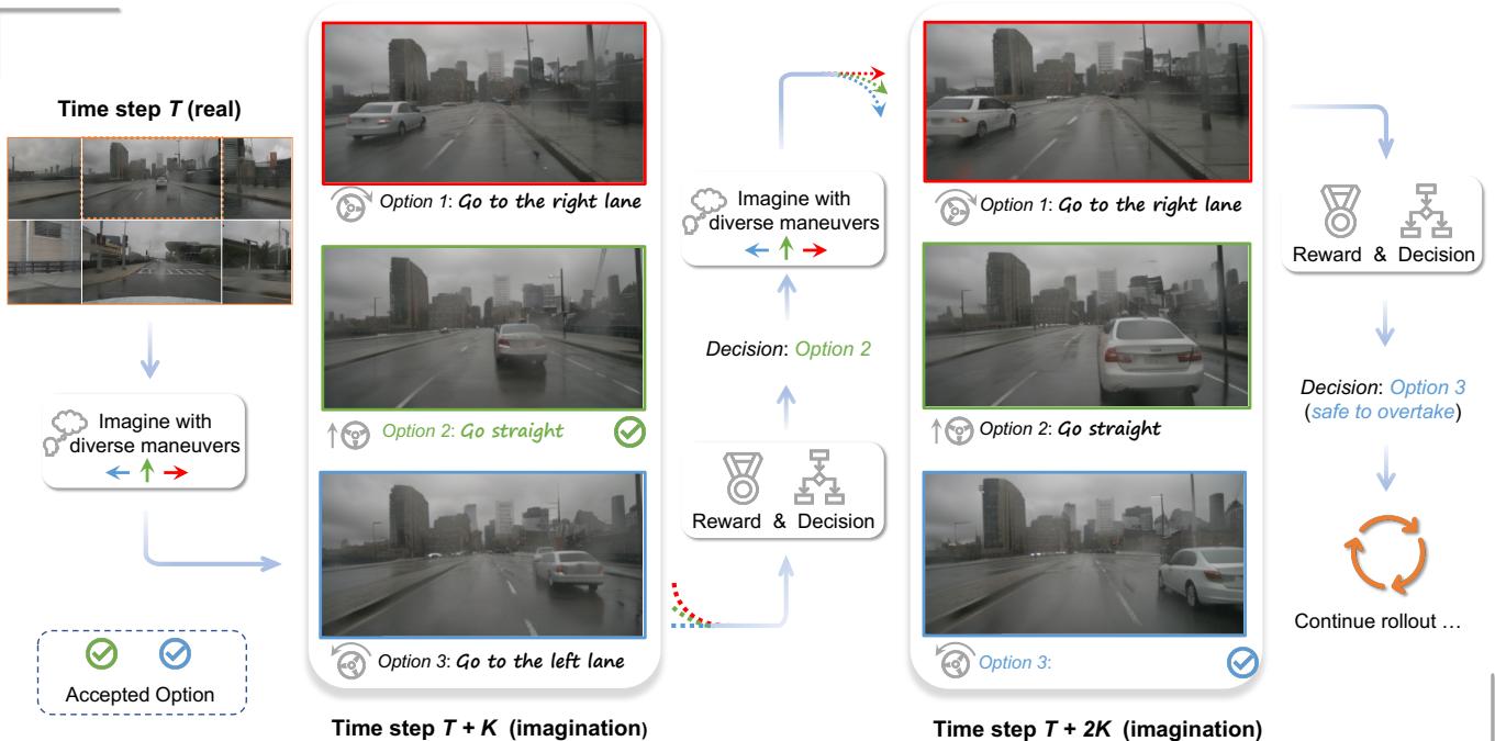
Figure 1. Multiview visual forecasting and planning by world model. At time step $T$ , the world model imagines the multiple futures at $T+K$ , and finds it is safe to keep going straight at $T$ . Then the model realizes that the ego car will be too close to the front car according to the imagination of time step $T+2K$ , so it decides to change to the left lane for a safe overtaking.

Abstract

In autonomous driving, predicting future events in advance and evaluating the foreseeable risks empowers autonomous vehicles to better plan their actions, enhancing safety and efficiency on the road. To this end, we propose Drive-WM, the first driving world model compatible with existing end-to-end planning models. Through a joint spatialtemporal modeling facilitated by view factorization, our model generates high-fidelity multiview videos in driving scenes. Building on its powerful generation ability, we showcase the potential of applying the world model for safe driving planning for the first time. Particularly, our Drive-WM enables driving into multiple futures based on distinct driving maneuvers, and determines the optimal trajectory according to the image-based rewards. Evaluation on real-world driving datasets verifies that our method could generate high-quality, consistent, and controllable multiview videos, opening up possibilities for real-world simulations and safe planning.

1. Introduction

The emergence of end-to-end autonomous driving [29, 30, 54] has recently garnered increasing attention. These approaches take multi-sensor data as input and directly output planning results in a joint model, allowing for joint optimization of all modules. However, it is questionable whether an end-to-end planner trained purely on expert

驶向未来：用于自动驾驶的世界模型多视角视觉预测与规划

Yuqi Wang1∗ Jiawei He1∗ Lue Fan1∗ Hongxin ${\mathrm{Li}}^{1\ast }$ Yuntao Chen2B Zhaoxiang Zhang1,2B1中科院自动化研究所 2中国科学院人工智能研究院, 香港中文大学信息工程学院, 中科院自动化研究所项目页面:

https://drive-wm.github.io代码: https://github.com/BraveGroup/Drive-WM

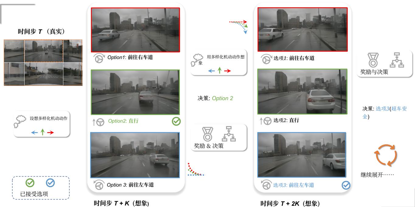
图 1。通过世界模型的多视角视觉预测与规划。在时间步 $T$ ，世界模型在 $T+K$ 想象出多种未来，并发现 $T$ 处继续直行是安全的。随后模型根据时间步 $T+2K$ 的想象意识到自车会与前车距离过近，因此决定换到左车道以安全完成超车。

摘要

在自动驾驶中，提前预测未来事件并评估可预见的风险，使自动驾驶车辆能够更好地规划其动作，从而提升道路上的安全性和效率。为此，我们提出了Drive-WM，这是首个与现有端到端规划模型兼容的驾驶世界模型。通过由视图分解促进的联合时空建模，我们的模型能在驾驶场景中生成高保真度的多视角视频。基于其强大的生成能力，我们首次展示了将该世界模型用于安全驾驶规划的潜力。具体而言，我们的Drive-WM 能够基于

识别出不同的驾驶动作，并根据基于图像的奖励确定最优轨迹。在真实驾驶数据集上的评估验证了我们的方法能够生成高质量、一致且可控的多视角视频，为真实世界模拟和安全规划打开了可能性。

1. 引言

端到端自动驾驶的出现 [29, 30,54]最近引起了越来越多的关注。这类方法以多传感器数据为输入，在一个联合模型中直接输出规划结果，从而允许对所有模块进行联合优化。然而，仅以专家

driving trajectories has sufficient generalization capabilities when faced with out-of-distribution (OOD) cases. As illustrated in Figure 2, when the ego vehicle’s position deviates laterally from the center line, the end-to-end planner struggles to generate a reasonable trajectory. To alleviate this problem, we propose improving the safety of autonomous driving by developing a predictive model that can foresee planner degradation before decision-making. This model, known as a world model [19, 20, 35], is designed to predict future states based on current states and ego actions. By visually envisioning the future in advance and obtaining feedback from different futures before actual decision-making, it can provide more rational planning, enhancing generalization and safety in end-to-end autonomous driving.

However, learning high-quality world models compatible with existing end-to-end autonomous driving models is challenging, despite successful attempts in game simulations [19–21, 46] and laboratory robotics environments [12, 20]. Specifically, there are three main challenges: (1) The driving world model requires modeling in high-resolution pixel space. The previous low-resolution image [20] or vectorized state space [4] methods cannot effectively represent the numerous fine-grained or non-vectorizable events in the real world. Moreover, vector space world models need extra vector annotations and suffer from state estimation noise of perception models. (2) Generating multiview consistent videos is difficult. Previous and concurrent works are limited to single view video [28, 31, 63] or multiview image generation [17, 53, 69], leaving multiview video generation an open problem for comprehensive environment observation needed in autonomous driving. (3) It is challenging to flexibly accommodate various heterogeneous conditions like changing weather, lighting, ego actions, and road/obstacle/vehicle layouts.

To address these challenges, we propose Drive-WM. Inspired by latent video diffusion models [2, 13, 48, 73], we introduce multiview and temporal modeling for jointly generating multiple views and frames. To further enhance multiview consistency, we propose factorizing the joint modeling to predict intermediate views conditioned on adjacent views, greatly improving consistency between views. We also introduce a simple yet effective unified condition interface enabling flexible use of heterogeneous conditions like images, text, 3D layouts, and actions, greatly simplifying conditional generation. Finally, building on the multiview world model, we explore end-to-end planning applications to enhance autonomous driving safety, as shown in Figure 1. The main contributions of our work can be summarized as follows.

• We propose Drive-WM, a multiview world model, which is capable of generating high-quality, controllable, and consistent multiview videos in autonomous driving scenes.

(a) Planning with ego on centerline (b) Planning with ego off centerline
Figure 2. Ego vehicle’s slight deviation from centerline causes motion planner to struggle generating reasonable trajectories. We shift the ego location $0.5\mathrm{m}$ to the right to create an out-ofdomain case. (a) shows the reasonable trajectory prediction of the VAD [30] method under normal data, and (b) shows the irrational trajectory when encountering out-of-distribution cases.

• Extensive experiments on the nuScenes dataset showcase the leading video quality and controllability. Drive-WM also achieves superior multiview consistency, evaluated by a novel keypoint matching based metric. • We are the first to explore the potential application of the world model in end-to-end planning for autonomous driving. We experimentally show that our method could enhance the overall soundness of planning and robustness in out-of-distribution situations.

2. Related Works

2.1. Video Generation and Prediction

Video generation aims to generate realistic video samples. Various generation methods have been proposed in the past, including VAE-based (Variational Autoencoder) [16, 33, 58, 61], GAN-based (generative adversarial networks) [3, 15, 31, 49, 56, 70], flow-based [10, 34] and auto-regressive models [18, 64, 68]. Notably, the recent success of diffusion-based models in the realm of image generation [40, 44, 45] has ignited growing interest in applying diffusion models to the realm of video generation [23, 26]. Diffusion-based methods have yielded significant enhancements in realism, controllability, and temporal consistency. Text-conditional video generation has garnered more attention due to its controllable generation, and a plethora of methods have emerged [2, 25, 48, 66, 73].

Video prediction can be regarded as a special form of generation, leveraging past observations to anticipate future frames [1, 9, 22, 26, 41, 59, 60, 65]. Especially in autonomous driving, DriveGAN [31] learns to simulate a driving scenario with vehicle control signals as its input. GAIA1 [28] and DriveDreamer [63] further extend to actionconditional diffusion models, enhancing the controllability and realism of generated videos. However, these previous works are limited to monocular videos and fail to comprehend the overall 3D surroundings. We have pioneered the generation of multiview videos, allowing for better integration with current BEV perception and planning models.

驾驶轨迹训练的端到端规划器在面对分布外（OOD）情况时是否具有足够的泛化能力仍值得怀疑。如图2所示，当自车位置在横向上偏离中心线时，端到端规划器难以生成合理的轨迹。为缓解这一问题，我们提出通过开发一种能够在决策前预见规划器退化的预测模型来提升自动驾驶的安全性。该模型，称为世界模型[19,20,35],，旨在基于当前状态和自车动作预测未来状态。通过在实际决策前可视化地预见未来并从不同未来中获取反馈，它能够提供更为合理的规划，增强端到端自动驾驶的泛化能力和安全性。

然而，尽管在游戏仿真[19–21,46]和实验室机器人环境[12,20]中已有成功尝试，学习与现有端到端自动驾驶模型兼容的高质量世界模型仍然具有挑战性。具体来说，存在三大主要挑战：(1) 驾驶世界模型需要在高分辨率像素空间中建模。以往的低分辨率图像[20]或向量化状态空间 [4]方法无法有效表示现实世界中大量细粒度或不可向量化的事件。此外，向量空间世界模型需要额外的向量注释，并且受到感知模型状态估计噪声的影响。(2) 生成多视角一致性视频困难。以往和同时期的工作仅限于单视角视频 [28, 31, 63]或多视角图像生成 [17, 53, 69], ，而多视角视频生成仍是一个开放问题，而全面环境观测对自动驾驶至关重要。(3) 灵活适应各种异质条件具有挑战性，例如变化的天气、光照、自车动作以及道路/障碍物/车辆布局。

为了解决这些挑战，我们提出了 Drive‑WM。受潜在视频扩散模型启发 [2, 13, 48, 73], ，我们引入了多视角和时间建模，用于联合生成多视角和多帧。为进一步增强多视角一致性，我们提出将联合建模分解为在相邻视角条件下预测中间视角，从而大大提高视角之间的一致性。我们还引入了一个简单但有效的统一条件接口，能够灵活使用图像、文本、三维布局和动作等异构条件，极大地简化条件生成。最后，基于多视角世界模型，我们探索了端到端规划应用以提升自动驾驶安全性，如图1所示。我们工作的主要贡献可归纳如下。

•我们提出了 Drive‑WM，一种多视角世界模型，能够在自动驾驶场景中生成高质量、可控且一致的多视角视频。

(a) 自车在中心线上规划 (b) 自车偏离中心线时的规划
图 2. 自车相对于中心线的轻微偏移会导致运动规划器难以生成合理的轨迹。我们将自车位置向右移动 $0.5\mathrm{m}$ ，创造了一个分布外的情况。(a) 展示了 VAD [30] 方法在正常数据下的合理轨迹预测，(b) 展示了在遇到分布外样例时的不合理轨迹。

• 在 nuScenes 数据集上进行的大量实验展示了领先的视频质量和可控性。Drive‑WM 在由一种基于关键点匹配的新度量评估的多视角一致性方面也表现优异。

• 我们是首个探索世界模型在自动驾驶端到端规划中潜在应用的工作。实验证明我们的方法能够提升规划的整体合理性并在分布外情形中增强鲁棒性。

2. Related Works

2.1. Video Generation and Prediction

视频生成旨在生成真实的视频样本。过去提出了多种生成方法，包括基于VAE（变分自编码器）的[16, 33, 58, 61], 、基于GAN（生成对抗网络）的[3, 15, 31, 49, 56, 70], 、基于流的方法 [10, 34]以及自回归模型 [18, 64, $68{]}_{\circ }$ 。值得注意的是，扩散模型在图像生成领域的近期成功 [40, 44, 45] 激发了人们将扩散模型应用于视频生成领域的兴趣[23,26]。基于扩散的方法在真实感、可控性和时间一致性方面带来了显著提升。由于其可控的生成能力，文本条件视频生成受到了更多关注，并涌现了大量方法 [2, 25, 48, 66, 73]。

视频预测可以被视为一种特殊的生成形式，利用过去的观测来预测未来帧 [1, 9, 22, 26, 41, 59, 60, $65\mathrm{lo}$ 尤其在自动驾驶中，DriveGAN [31] 学会以车辆控制信号作为输入来模拟驾驶场景。GAIA‑1 [28]和DriveDreamer [63] 进一步扩展到基于动作条件的扩散模型，提升了生成视频的可控性和真实感。然而，这些先前工作仅限于单目视频，无法理解整体的三维环境。我们率先提出多视角视频的生成，使其能够更好地与当前的鸟瞰图感知和规划模型集成。

2.2. World Model for Planning

The world model [35] learns a general representation of the world and predicts future world states resulting from a sequence of actions. Learning world models in either game [19–21, 43, 47] or lab environments [12, 14, 67] has been widely studied. Dreamer [20] learns a latent dynamics model from past experience to predict state values and actions in a latent space. It is capable of handling challenging visual control tasks in the DeepMind Control Suite [55]. DreamerV2 [21] improves upon Dreamer to achieve human-level performance on Atari games. DreamerV3 [22] uses larger networks and learns to obtain diamonds in Minecraft from scratch given sparse rewards, which is considered a long-standing challenge. DayDreamer [67] applies Dreamer [20] to training 4 robots online in the real world and solves locomotion and manipulation tasks without changing hyperparameters. Recently, learning world models in driving scenes has gained attention. MILE [27] employs a model-based imitation learning method to jointly learn a dynamics model and driving behaviour in CARLA [11]. The aforementioned works are limited to either simulators or well-controlled lab environments. In contrast, our world model can be integrated with existing end-to-end driving planners to improve planning performance in real-world scenes.

3. Multi-view Video Generation

In this section, we first present how to jointly model the multiple views and frames, which is presented in Sec 3.1. Then we enhance multiview consistency by factorizing the joint modeling in Sec 3.2. Finally, Sec. 3.3 elaborates on how we build a unified condition interface to integrate the multiple heterogeneous conditions.

3.1. Joint Modeling of Multiview Video

To jointly model multiview temporal data, we start with the well-studied image diffusion model and adapt it into multiview-temporal scenarios by introducing additional temporal layers and multiview layers. In this subsection, we first present the overall formulation of joint modeling and elaborate on the temporal and multiview layers.

Formulation. We assutiview videos, such that $p_{\mathrm{data}}$ $\mathbf{x}\in {\mathbb{R}}^{T\times K\times 3\times H\times W}$ $\mathbf{x}\sim p_{\mathrm{data}}$ is a sequence of $T$ images with $K$ views, with height and width $H$ and $W$ . Given encoded video latent representation $\mathcal{E}(\mathbf{x})=\mathbf{z}\in {\mathbb{R}}^{T\cdot K\times C\times \hat{H}\times \hat{W}}$ , diffused inputs ${\mathbf{z}}_{\tau }={\alpha }_{\tau }\mathbf{z}+{\sigma }_{\tau }ϵ$ , $ϵ\sim \mathcal{N}(0,I)$ , here ${\alpha }_{\tau }$ and ${\sigma }_{\tau }$ define a noise schedule parameterized by a diffusion time step $\tau$ . A denoising model ${\mathbf{f}}_{\theta ,\varphi ,\psi }$ (parameterized by spatial parameters $\theta$ , temporal parameters $\varphi$ and multiview parameters $\psi$ )

receives the diffused ${\mathbf{z}}_{\tau }$ as input and is optimized by minimizing the denoising score matching objective

$${\mathbb{E}}_{\mathbf{z}\sim p_{\mathrm{data}},\tau \sim p_{\tau },ϵ\sim \mathcal{N}(0,I)}[\Vert \mathbf{y}-{\mathbf{f}}_{\theta ,\varphi ,\psi }({\mathbf{z}}_{\tau };\mathbf{c},\tau ){\Vert }_2^2],$$

where $\mathbf{c}$ is the condition, and target $\mathbf{y}$ is the random noise $ϵ$ .
$p_{\tau }$ is a uniform distribution over the diffusion time $\tau$ .

Temporal encoding layers. We first introduce temporal layers to lift the pretrained image diffusion model into a temporal model. The temporal encoding layer is attached after the 2D spatial layer in each block, following established practice in VideoLDM [2]. The spatial layer encodes the latent $\mathbf{z}\in {\mathbb{R}}^{T\cdot K\times C\times \hat{H}\times \hat{W}}$ in a frame-wise and viewwise manner. Afterward, we rearrange the latent to hold out the temporal dimension, denoted as (TK) $\mathrm{CHW}\to \mathrm{KCTHW}$ , to apply the 3D convolution in spatio-temporal dimensions THW. Then we arrange the latent to (KHW)TC and apply standard multi-head self-attention to the temporal dimension, enhancing the temporal dependency. The notation $\varphi$ in Eq. 1 stands for the parameters of this part.

Multiview encoding layers. To jointly model the multiple views, there must be information exchange between different views. Thus we lift the single-view temporal model to a multi-view temporal model by introducing multiview encoding layers. In particular, we rearrange the latent as (KHW) $\begin{array}{rl}\mathrm{TC}& (\mathrm{TH}\bar{\mathsf{W}})\mathrm{KC}\end{array}$ to hold out the view dimension. Then a self-attention layer parameterized by $\psi$ in Eq. 1 is employed across the view dimension. Such multiview attention allows all views to possess similar styles and consistent overall structure.

Multiview temporal tuning. Given the powerful image diffusion models, we do not train the temporal multiview network from scratch. Instead, we first train a standard image diffusion model with single-view image data and conditions, which corresponds to the parameter $\theta$ in Eq. 1. Then we freeze the parameters $\theta$ and fine-tune the additional temporal layers $(\varphi )$ and multiview layers $(\psi )$ with video data.

3.2. Factorization of Joint Multiview Modeling

Although the joint distributions in Sec. 3.1 could yield similar styles between different views, it is hard to ensure strict consistency in their overlapped regions. In this subsection, we introduce the distribution factorization to enhance multiview consistency. We first present the formulation of factorization and then describe how it cooperates with the aforementioned joint modeling.

Formulation. Let ${\mathbf{x}}_i$ denote the sample of $i$ -th view, Sec. 3.1 essentially model the joint distribution $p({\mathbf{x}}_{1,\dots ,K})$ , which can be into

$$p({\mathbf{x}}_{1,\dots ,K})=p({\mathbf{x}}_1)p({\mathbf{x}}_2|{\mathbf{x}}_1)\dots p({\mathbf{x}}_K|{\mathbf{x}}_1,\dots ,{\mathbf{x}}_{K-1}).$$

2.2. 规划的世界模型

The worldmodel [35] 学习世界的一般表示，并预测由一系列动作导致的未来世界状态。在游戏 [19–21, 43, 47]或实验室环境中 [12, 14, 67]学习世界模型已被广泛研究。Dreamer [20] 从过去经验中学习潜在动态模型，以在潜在空间中预测状态值和动作。它能够处理 DeepMind 控制套件 [55]中的具有挑战性的视觉控制任务。DreamerV2 [21] 在 Dreamer 基础上改进，达到了 Atari 游戏的人类级表现。DreamerV3 [22]使用更大的网络并从零开始在Minecraft 中学习在稀疏奖励下获取钻石，这被视为一个长期的挑战。Day‑ Dreamer [67]将 Dreamer [20]应用于真实世界中对 4 台机器人进行在线训练，并在不改变超参数的情况下解决了移动和操控任务。最近，在驾驶场景中学习世界模型受到关注。MILE [27]采用一种基于模型的模仿学习方法，在 CARLA 中联合学习动力学模型和驾驶行为 [11]。上述工作要么局限于模拟器，要么局限于受控的实验室环境。相比之下，我们的世界模型可以与现有的端到端驾驶规划器集成，以提升真实场景中的规划性能。

3. 多视角视频生成

在本节中，我们首先介绍如何联合建模多个视图和帧，内容见第3.1节。然后我们通过在第3.2节对联合建模进行因式分解来增强多视角一致性。最后，第3.3 节阐述了我们如何构建统一条件接口以整合多种异构条件。

3.1. 多视角视频的联合建模

为了对多视角时序数据进行联合建模，我们从已有的图像扩散模型出发，通过引入额外的时序层和多视角层将其适配到多视角‑时序场景。在本小节中，我们首先给出联合建模的整体表述，并详细说明时序层和多视角层。

公式说明。 我们假设可以访问一个数据集 $p_{\mathrm{data}}$ ，由多视图视频组成，使得 $\mathbf{x}\in {\mathbb{R}}^{T\times K\times 3\times H\times W},$ 、 $\mathbf{x}\sim p_{\mathrm{data}}$ 是一系列包含 $T$ 张具有 $K$ 个视图的图像，具有高度和宽度 $H$ 和 $W$ 。给定编码后的视频潜变量表示

$\mathcal{E}(\mathbf{x})=\mathbf{z}\in {\mathbb{R}}^{T\cdot K\times C\times \hat{H}\times \hat{W}}.$ 、扩散后的输入$\begin{array}{r}{\mathbf{z}}_{\tau }={\alpha }_{\tau }\mathbf{z}+{\sigma }_{\tau }\mathbf{ϵ}\mathbf{ϵ}\sim \mathcal{N}(0,\mathbf{I}),\end{array}$ ，此处 ${\alpha }_{\tau }$ 和 ${\sigma }_{\tau }$ 由由扩散时间步 $\tau$ 参数化的噪声调度定义。一个去噪模型 ${\mathbf{f}}_{\theta \varphi \psi }$ ,(由空间参数 $\theta .$ 、时序参数 $\varphi$ 和多视图参数 $\psi$ 参数化)

接收作为输入的扩散 $\mathbf{z}\tau$ 并通过最小化去噪评分匹配目标进行优化

$${\mathbb{E}}_{\mathbf{z}\sim p_{\mathrm{data}},\tau \sim p_{\tau },ϵ\sim \mathcal{N}(0,I)}[\Vert \mathbf{y}-{\mathbf{f}}_{\theta ,\varphi ,\psi }({\mathbf{z}}_{\tau };\mathbf{c},\tau ){\Vert }_2^2],$$

其中c 是条件，目标y 是随机噪声 ${ϵ}_{\circ }{p}_{\tau }$ 是在扩散时间 $\tau$ 上的均匀分布。

时序编码层。 我们首先引入 时序层 以将预训练的图像扩散模型提升为时序模型。时序编码层附加在每个模块中的二维空间层之后，遵循 VideoLDM 的既定做法 $[2{]}_{\circ }$ 。空间层以逐帧且逐视图的方式对潜变量进行编码 $\mathbf{z}\in {\mathbb{R}}^{T\cdot K\times C\times \hat{H}\times \hat{W}}$ 。随后，我们重新排列潜变量以保留时间维度，记作 (TK) $\complement \mathrm{H}\vee ⟹\mathrm{KCTHW}$ ，以在时空维度上应用三维卷积THW。然后我们将潜变量重新排列为 (KHW)TC 并对时间维度应用标准的多头自注意力，从而增强时间依赖性。符号 $\varphi$ 在式1 中表示该部分的参数。

多视角编码层。 为了联合建模多个视图，不同视图之间必须进行信息交换。因此我们通过引入 多视角编码层将单视图时序模型提升为多视角时序模型。具体来说，我们将潜变量重新排列为(KHW)TC

(THW)KC 以保留视图维度。然后使用由 $\psi$ 在式1 中参数化的自注意力层跨视图维度进行操作。这样的多视角注意力使所有视图具有相似的风格和一致的整体结构。

多视角时序微调。 鉴于强大的图像扩散模型，我们并不是从头训练时序多视角网络。相反，我们首先使用单视角图像数据和条件训练一个标准的图像扩散模型，这对应于参数 $\theta$ 在公式 1 中。然后我们冻结参数 $\theta$ 并使用视频数据微调附加的时序层 $(\varphi )$ ）和多视角层 $(\psi )$ ）。

3.2. 联合多视角建模的因式分解

尽管第 3.1节中的联合分布可以在不同视图之间产生相似的风格，但难以在它们重叠的区域确保严格一致性。在本小节中，我们引入分布因式分解以增强多视角一致性。我们首先给出因式分解的表述，然后描述其如何与前述的联合建模协同工作。

表述。设 ${\mathbf{x}}_i$ 表示第 $i$ 个视图的样本，见第3.1 节，实质上对联合分布进行建模 $p({\mathbf{x}}_{1,\dots ,K})$ ，其可以被分解为

$$p({\mathbf{x}}_{1,\dots ,K})=p({\mathbf{x}}_1)p({\mathbf{x}}_2|{\mathbf{x}}_1)\dots p({\mathbf{x}}_K|{\mathbf{x}}_1,\dots ,{\mathbf{x}}_{K-1}).$$

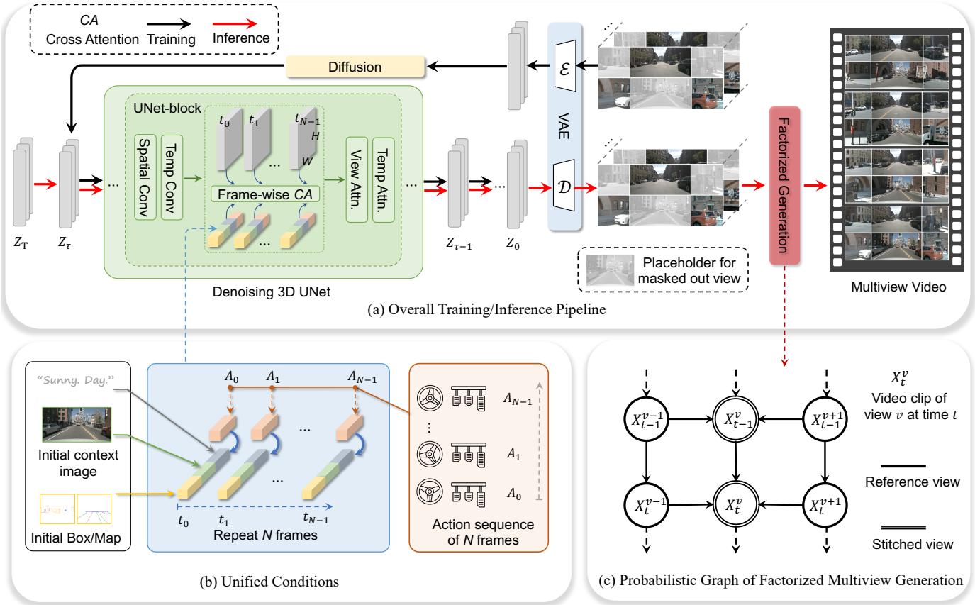
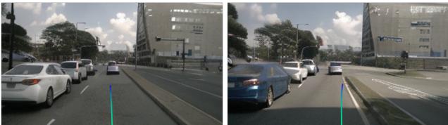
Figure 3. Overview of the proposed framework. (a) illustrates the training and inference pipeline of the proposed method. (b) visualizes the unified conditions leveraged to control the generation of multi-view video. © represents the probabilistic graph of factorized multiview generation. It takes the 3-view output from (a) as input to generate other views, enhancing the multi-view consistency.

Eq. 2 indicates that different views are generated in an autoregressive manner, where a new view is conditioned on existing views. These conditional distributions can ensure better view consistency because new views are aware of the content in existing views. However, such an autoregressive generation is inefficient, making such full factorization infeasible in practice.

To simplify the modeling in Eq. 2, we partition all views into two types: reference views ${\mathbf{x}}_r$ and stitched views ${\mathbf{x}}_s$ . For example, in nuScenes, reference views can be the {F,BL,BR}\left\{ \mathrm { F } , \quad \mathrm { B L } , \quad \mathrm { B R } \right\}{F,BL,BR} , and stitched views can be {FL,B,FR}\left\{ { \mathrm { F L } } , \quad { \mathrm { B } } , \quad { \mathrm { F R } } \right\}{FL,B,FR} . We use the term “stitched” because a stitched view appears to be “stitched” from its two neighboring reference views. Views belonging to the same type do not overlap with each other, while different types of views may overlap. This inspires us to first model the joint distribution of reference views. Here the joint modeling is effective for those non-overlapped reference views since they do not necessitate strict consistency. Then the distribution of ${\mathbf{x}}_s$ is modeled as a conditional distribution conditioned on the ${\mathbf{x}}_r$ . Figure 4 illustrates the basic concept of multiview factorization in nuScenes. In this sense, we

simplify Eq. 2 into

$$p(\mathbf{x})=p({\mathbf{x}}_s,{\mathbf{x}}_r)=p({\mathbf{x}}_r)p({\mathbf{x}}_s|{\mathbf{x}}_r).$$

Considering the temporal coherence, we incorporate previous frames as additional conditions. The Eq. 3 can be re-written as

$$p(\mathbf{x})=p({\mathbf{x}}_s,{\mathbf{x}}_r|{\mathbf{x}}_{pre})=p({\mathbf{x}}_r|{\mathbf{x}}_{pre})p({\mathbf{x}}_s|{\mathbf{x}}_r,{\mathbf{x}}_{pre}),$$

where ${\mathbf{x}}_{pre}$ is context frames (e.g., the last two frames) from previously generated video clips. The distribution of reference views $p({\mathbf{x}}_r|{\mathbf{x}}_{pre})$ is implemented by the pipeline in Sec. 3.1. As for $p({\mathbf{x}}_s|{\mathbf{x}}_r,{\mathbf{x}}_{pre})$ , we adopt the similar pipeline but incorporate neighboring reference views as an additional condition as Figure 4 shows. We introduce how to use conditions in the following subsection.

3.3. Unified Conditional Generation

Due to the great complexity of the real world, the world model needs to leverage multiple heterogeneous conditions. In our case, we utilize initial context frames, text descriptions, ego actions, 3D boxes, BEV maps, and reference views. More conditions can be further included for better 式2 表明不同视图以自回归的方式生成，新视图以已 有视图为条件。这些条件分布能够保证更好的视图一 致性，因为新视图会考虑已有视图中的内容。然而， 这种自回归生成效率低下，使得在实践中进行这种完 全因子分解不可行。

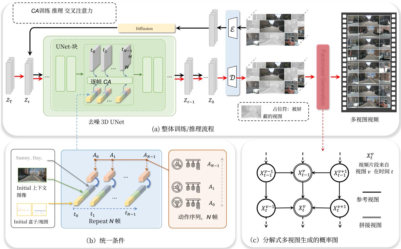
图3。所提出框架的概览。（a）展示了所提出方法的训练与推理流程。(b)可视化了用于控制多视角视频生成的统一条件。©表示分解式多视角生成的概率图。它以（a）中的三视图输出作为输入来生成其他视图，以增强多视角一致性。

为简化式2中的建模，我们将所有视图划分为两类：参考视图 $\mathbf{x}r$ 和拼接视图 ${\mathbf{x}}_{s_0}$ 。例如，在 nuScenes 中，参考视图可以是 {F, BL, $\mathtt{BR}{\}}^2$ ，而拼接视图可以是{FL, B, FR}。我们使用“拼接”一词是因为拼接视图看起来像是从其两个相邻的参考视图“拼接”而成。同一类型的视图之间不重叠，而不同类型的视图则可能重叠。这启发我们先对参考视图的联合分布进行建模。这里对那些不重叠的参考视图进行联合建模是有效的，因为它们无需严格一致性。然后将 ${\mathbf{\Delta }}_{\mathbf{x}s}$ 的分布建模为条件于 $\mathbf{x}r$ 的条件分布。图4说明了 nuScenes 中多视图分解的基本概念。从这个意义上讲，我们

将式2 简化为

$$p(\mathbf{x})=p({\mathbf{x}}_s,{\mathbf{x}}_r)=p({\mathbf{x}}_r)p({\mathbf{x}}_s|{\mathbf{x}}_r).$$

考虑到时序一致性，我们将之前的帧作为额外条件纳入。等式3 可以重写为

$$p(\mathbf{x})=p({\mathbf{x}}_s,{\mathbf{x}}_r|{\mathbf{x}}_{pre})=p({\mathbf{x}}_r|{\mathbf{x}}_{pre})p({\mathbf{x}}_s|{\mathbf{x}}_r,{\mathbf{x}}_{pre}),$$

其中xpre 是来自先前生成的视频片段的上下文帧（例如，最近两帧）。参考视图的分布 $p({\mathbf{x}}_r|{\mathbf{x}}_{pre})$ 由第3.1节中的流程实现。至于 $p({\mathbf{x}}_s|{\mathbf{x}}_r,{\mathbf{x}}_{pre})$ ，我们采用类似的流程，但将相邻参考视图作为额外条件并入，如图4所示。下节中我们将介绍如何使用这些条件。

3.3. 统一条件生成

由于现实世界的高度复杂性，世界模型需要利用多种异构条件。在我们的场景中，我们使用了初始上下文帧、文本描述、自车动作、3D 立方体、鸟瞰图（BEV）和参考视图。还可以进一步加入更多条件以获得更好的

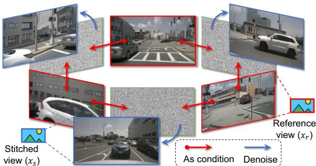
Figure 4. Illustration of factorized multi-view generation. We take the sensor layout in nuScenes as an example.

controllability. Developing specialized interface for each one is time-consuming and inflexible to incorporate more conditions. To address this issue, we introduce a unified condition interface, which is simple yet effective in integrating multiple heterogeneous conditions. In the following, we first introduce how we encode each condition, and then describe the unified condition interface.

Image condition. We treat initial context frames (i.e., the first frame of a clip) and reference views as image conditions. A given image condition $\text{ I }\in {\mathbb{R}}^{3\times H\times W}$ is encoded and flattened to a sequence of $d$ -dimension embeddings $\mathbf{i}=(i_1,i_2,...,i_n)\in {\mathbb{R}}^{n\times d}$ , using ConvNeXt as encoder [39]. Embeddings from different images are concatenated in the first dimension of $n$ .

Layout condition. Layout condition refers to 3D boxes, HD maps, and BEV segmentation. For simplicity, we project the 3D boxes and HD maps into a 2D perspective view. In this way, we leverage the same strategy with image condition encoding to encode the layout condition, resulting in a sequence of embeddings $\mathbf{l}=(l_1,l_2,...,l_k)\in {\mathbb{R}}^{k\times d}$ . $k$ is the total number of embeddings from the projected layouts and BEV segmentation.

Text condition. We follow the convention of diffusion models to adopt a pre-trained CLIP [42] as the text encoder. Specifically, we combine view information, weather, and light to derive a text description. The embeddings are denoted as $\mathbf{e}=(e_1,e_2,...,e_m)\in {\mathbb{R}}^{m\times d}$ .

Action condition. Action conditions are indispensable for the world model to generate the future. To be compatible with the existing planning methods [30], we define the action in a time step as $(\Delta x,\Delta y)$ , which represents the movement of ego location to the next time step. We use an MLP to map the action into a $d$ -dimension embedding $\mathbf{a}\in {\mathbb{R}}^{2\times d}$

A unified condition interface. So far, all the conditions are mapped into $d$ -dimension feature space. We take the concatenation of required embeddings as input for the denoising UNet. Taking action-based joint video generation as an example, this allows us to utilize the initial context images, initial layout, text description, and frame-wise action sequence. So we have unified condition embeddings in a certain time $t$ as

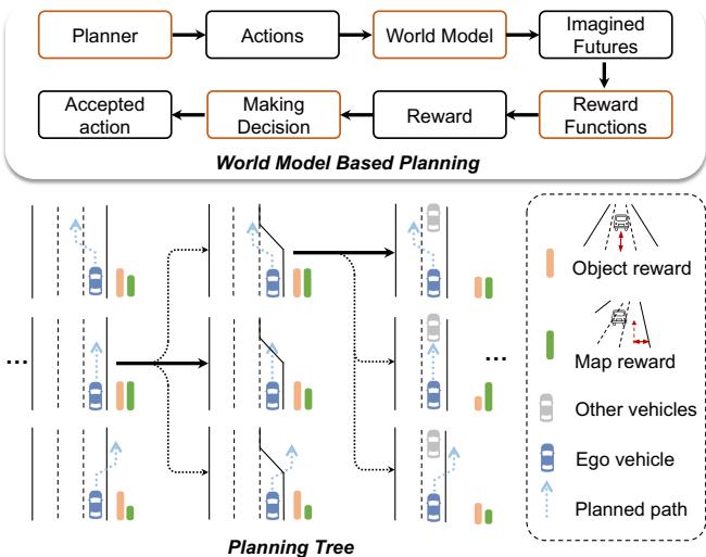
Figure 5. End-to-end planning pipeline with our world model. We display the components of our planning pipeline at the top and illustrate the decision-making process in the planning tree using image-based rewards at the bottom.

$${\mathbf{c}}_t=[{\mathbf{i}}_0,{\mathbf{l}}_0,{\mathbf{e}}_0,{\mathbf{a}}_t]\in {\mathbb{R}}^{(n+k+m+2)\times d},$$

where subscript $t$ stands for the $t$ -th generated frame and subscript 0 stands for the current real frame. We emphasize that such a combination of different conditions offers a unified interface and can be adjusted by the request. Finally, ${\mathbf{c}}_{\mathbf{t}}$ interacts with the latent ${\mathbf{z}}_{\mathbf{t}}$ in 3D UNet by cross attention in a frame-wise manner (Figure 3 (a)).

4. World Model for End-to-End Planning

Blindly planning actions without anticipating consequences is dangerous. Leveraging our world model enables comprehensive evaluation of possible futures for safer planning. In this section, we explore end-to-end planning using the world model for autonomous driving, an uncharted area.

4.1. Tree-based Rollout with Actions

We describe planning with world models in this section. At each time step, we leverage the world model to generate predicted future scenarios for trajectory candidates sampled from the planner, evaluate the futures using an image-based reward function, and select the optimal trajectory to extend the planning tree.

As shown in Figure 5, we define the planning tree as a series of predicted ego trajectories that evolve over time. For each time, the real multiview images can be captured by the camera. The pre-trained planner takes the real multiview images as input and samples possible trajectory candidates. To be compatible with the input of mainstream planner, we define its action ${\mathbf{a}}_{\mathbf{t}}$ at time $t$ as $(x_{t+1}-x_t,y_{t+1}-y_t)$ for 可控性。为每种条件开发专门的接口既费时又在整合 更多条件时缺乏灵活性。为了解决这一问题，我们引 入了一个统一条件接口，该接口简单但在整合多种异 构条件方面非常有效。下面我们先介绍如何编码每种 条件，然后描述统一条件接口。

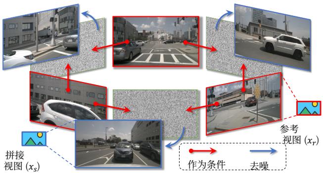
图4。因式分解多视角生成示意图。我们以 nuScenes 中的传感器布局为例。

图像条件。 我们将初始上下文帧（即片段的第一帧）和参考视图视为图像条件。给定的图像条件 $\text{ I }\in {\mathbb{R}}^{3\times H\times W}$ 被编码并展平为一系列 $d;$ 维嵌入

$\mathbf{i}=(i_1,i_2,...,i_n)\in {\mathbb{R}}^{n\times d}$ ，使用 ConvNeXt 作为编码器[39]。来自不同图像的嵌入在 $n$ 的第一个维度上连接。

布局条件。布局条件指 3D 立方体、高清地图 和 鸟瞰视图分割。为简单起见，我们将 3D 立方体和高清地图投影到二维透视视图中。通过这种方式，我们采用与图像条件编码相同的策略来编码布局条件，从而得到一个嵌入序列 $\mathbf{l}=(l_1,l_2,...,l_k)\in {\mathbb{R}}^{k\times d}$ 。 $k$ 是来自投影布局和鸟瞰视图分割的嵌入总数。

文本条件。我们遵循扩散模型的惯例，采用预训练的CLIP [42] 作为文本编码器。具体而言，我们将视图信息、天气和光照结合起来生成文本描述。该嵌入表示记为 $\mathbf{e}=(e_1,e_2,...,e_m)\in {\mathbb{R}}^{m\times d}{\mathrm{\Omega }}_{\mathrm{c}}$ 。

动作条件。动作条件对于世界模型生成未来是不可或缺的。为与现有规划方法 [30], 兼容，我们将一个时间步内的动作定义为 $(\Delta x,\Delta y)$ ，它表示自车位置从当前到下一个时间步的移动。我们使用一个多层感知器（MLP）将动作映射为一个 $d$ 维的嵌入 $\mathbf{a}\in {\mathbb{R}}^{2\times d}$ 。

统一条件接口。迄今为止，所有条件都被映射到 $d$ 维特征空间。我们将所需嵌入的拼接作为去噪UNet的输入。以基于动作的联合视频生成为例，这使我们能够利用初始上下文

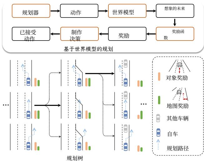
Figure 5. 使用我们的世界模型的端到端规划流水线。我们在上方展示了规划流水线的各个组件，并在下方用基于图像的奖励说明了规划树中的决策过程。

图像、初始布局、文本描述以及逐帧动作序列。因此我们在某个时间 $t$ 上具有统一的条件嵌入，作为

$${\mathbf{c}}_t=[{\mathbf{i}}_0,{\mathbf{l}}_0,{\mathbf{e}}_0,{\mathbf{a}}_t]\in {\mathbb{R}}^{(n+k+m+2)\times d},$$

其中下标 $t$ 表示第 $t$ 帧生成的 帧，且下标 0 表示当前的 真实 帧。我们强调，这种不同条件的组合提供了一个统一的接口，并可根据需求进行调整。最后， ${\mathbf{c}}_{\mathbf{t}}$ 在 3D UNet 中通过逐帧的交叉注意力与潜变量 ${\mathbf{z}}_{\mathbf{t}}$ 交互（图 3 (a)）。

4. 世界模型用于端到端规划

盲目地规划动作而不预见后果是危险的。利用我们的世界模型可以对可能的未来进行全面评估，从而实现更安全的规划。在本节中，我们探索了将世界模型用于自动驾驶的端到端规划，这是一个尚未充分涉足的领域。

4.1. 基于树的带动作展开

我们在本节描述了使用世界模型进行规划。在每个时间步，我们利用世界模型为从规划器采样的轨迹候选动作生成预测的未来场景，使用基于图像的奖励函数评估这些未来场景，并选择最佳轨迹以扩展规划树。

如图5所示，我们将规划树定义为随时间演化的一系列预测自车轨迹。对于每个时刻，摄像头可以捕获真实的多视角图像。预训练规划器以真实的多视角图像为输入并对可能的轨迹候选进行采样。为兼容主流规划器的输入，我们将其动作 ${\mathbf{a}}_{\mathbf{t}}$ 在时刻 $t$ 定义为

$(x_{t+1}-x_t,y_{t+1}-y_t)$ ，用于 each trajectory, where $x_t$ and $y_t$ are the ego locations at time $t$ . Given the actions, we adopt the condition combination in Eq. 5 for the video generation. After the generation, we leverage an image-based reward function to choose the optimal trajectory as the decision. Such a generation-decision process can be repeated to form a tree-based rollout.

4.2. Image-based Reward Function

After generating the future videos for planned trajectories, reward functions are required to evaluate the soundness of the multiple futures.

We first get the rewards from perception results. Particularly, we utilize image-based 3D object detector [37] and online HDMap predictor [38] to obtain the perception results on the generated videos. Then we define map reward and object reward, inspired by traditional planner [6, 30]. The map reward includes two factors, distance away from the curb, encouraging the ego vehicle to stay in the correct drivable area, and centerline consistency, preventing ego from frequently changing lanes and deviating from the lane in the lateral direction. The object reward means the distance away from other road users in longitudinal and lateral directions. This reward avoids the collision between the ego vehicle and other road users. The total reward is defined as the product of the object reward and the map reward. We finally select the ego prediction with the maximum reward. Then the planning tree forwards to the next timestamp and plans the subsequent trajectory iteratively.

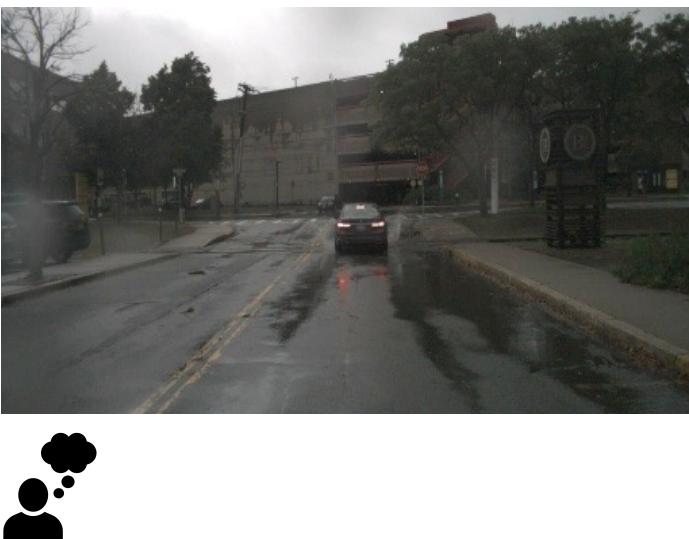
Since the proposed world model operates in pixel space, it can further get rewards from the non-vectorized representation to handle more general cases. For example, the sprayed water from the sprinkler and damaged road surface are hard to be vectorized by the supervised perception models, while the world model trained from massive unlabeled data could generate such cases in pixel space. Leveraging the recent powerful foundational models such as GPT-4V, the planning process can get more comprehensive rewards from the non-vectorized representation. In the appendix, we showcase some typical examples.

5. Experiments

5.1. Setup

Dataset. We adopt the nuScenes [5] dataset for experiments, which is one of the most popular datasets for 3D perception and planning. It comprises a total of 700 training videos and 150 validation videos. Each video includes around 20 seconds captured by six surround-view cameras. Training scheme. We crop and resize the original image from $1600\times 900$ to $384\times 192$ . Our model is initialized with Stable Diffusion checkpoints [44]. All experiments are conducted on A40 (48GB) GPUs. For additional details, please refer to the appendix.

Quality evaluation. To evaluate the quality of the generated video, we utilize FID (Frechet Inception Distance) [24] and FVD (Frechet Video Distance) [57] as the main metrics. Multiview consistency evaluation. We introduced a novel metric, the Key Points Matching (KPM) score, to evaluate multi-view consistency. This metric utilizes a pre-trained matching model [51] to calculate the average number of matching key points, thereby quantifying the KPM score. In the calculation process, for each image, we first compute the number of matched key points between the current view and its two adjacent views. Subsequently, we calculated the ratio between the number of matched points in generated data and the number of matched points in real data. Finally, we averaged these ratios across all generated images to obtain the KPM score. In practice, we uniformly selected 8 frames per scene in the validation set to calculate KPM.

Controllability evaluation. To assess the controllability of video content generation, we evaluate generated images using pre-trained perception models. Following the previous method [69], we adopted CVT [72] for foreground and background segmentation. Additionally, we evaluate 3D object detection [62] and online map construction [38].

Planning evaluation. We follow open-loop evaluation metrics [29, 30] for end-to-end planning, including L2 distance from the GT trajectory and the object collision rate.

Model variants. We support action-based video generation and layout-based video generation. The former gives the ego action of each frame as the condition, while the latter gives the layout (3D box, map information) of each frame.

5.2. Main Results of Multi-view Video Generation

We first demonstrate our superior generation quality and controllability. Here the generation is conditioned on frame-wise 3D layouts. Our model is trained in nuScenes train split, and evaluated with the conditions in val split.

Generation quality. Since we are the first one to explore multi-view video generation, we make separate comparisons with previous methods in multi-view images and single-view videos, respectively. For multi-view image generation, we remove the temporal layers in Sec. 3.1. Table 1a showcases the main results. In single-view image generation, we achieve 12.99 FID, achieving a significant improvement over previous methods. For video generation, our method exhibits a significant quality improvement compared to past single-view video generation methods, achieving 15.8 FID and 122.7 FVD. Additionally, our method is the first work to generate consistent multi-view videos, which is quantitatively demonstrated in Sec. 5.3.

Controllability. In Table 1b, we examine the controllabil-ity of our method on the nuScenes validation set. For fore-ground controllability, we evaluate the performance of 3D每条轨迹，其中 $x_t$ 和 $y_t$ 是时刻t的自车位置。给定这些动作，我们在式5中采用条件组合用于视频生成。生成完成后，我们利用基于图像的奖励函数来选择最优轨迹作为决策。这样的生成‑决策过程可以重复进行以形成基于树的展开。

4.2. 基于图像的奖励函数

在为规划轨迹生成未来视频后，需要奖励函数来评估这些多种未来情况的合理性。

我们首先从感知结果中获取奖励。具体而言，我们在生成的视频上使用基于图像的3D目标检测器 [37]和在线高清地图预测器 [38] 来获得感知结果。随后我们借鉴传统规划器，定义了地图奖励和对象奖励 [6, $30{\mathrm{J}}_{\mathrm{o}}$ 地图奖励包括两个因素：与路缘的距离，鼓励自车保持在正确的可通行区域，以及车道中心线一致性，防止自车频繁变道并在横向上偏离车道。对象奖励表示与其他道路使用者在纵向和横向方向上的距离，该奖励用于避免自车与其他道路使用者发生碰撞。总奖励定义为对象奖励与地图奖励的乘积。最终我们选择奖励最大的自车预测。随后规划树前进到下一个时间步，并迭代地规划后续轨迹。

由于所提出的世界模型在像素空间中运行，它还可以从非向量化表示中获得奖励，以处理更一般的情况。例如，喷水器喷出的水和损坏的路面很难被监督感知模型向量化，而从大量无标注数据训练的世界模型可以在像素空间中生成此类情况。利用近期强大的基础模型（如GPT‑4V），规划过程可以从非向量化表示中获得更全面的奖励。在附录中，我们展示了一些典型示例。

5. 实验

5.1. 设置

数据集。我们在实验中采用了 nuScenes [5] 数据集，该数据集是三维感知与规划中最常用的数据集之一。它包含共计 700 个训练视频和 150 个验证视频。每个视频包含由六个环视摄像头拍摄的约 20 秒的视频。训练方案。我们将原始图像从 $1600\times 900$ 裁剪并调整为 $384\times 192,$ 。我们的模型以 Stable Diffusion 检查点 [44]进行初始化。所有实验均在 A40（48GB）GPU 上完成。更多细节请参见附录。

质量评估。 为评估生成视频的质量，我们采用 FID（Frechet Inception Distance） [24] 和 FVD（Frechet Video Distance） [57] 作为主要指标。多视角一致性评估。 我们提出了一种新的指标——关键点匹配（KPM）分数，用于评估多视角一致性。该指标利用预训练的匹配模型 [51] 计算匹配关键点的平均数量，从而量化 KPM 分数。在计算过程中，对于每张图像，我们首先计算当前视图与其两个相邻视图之间的匹配关键点数量。随后，计算生成数据中匹配点数量与真实数据中匹配点数量的比值。最后，对所有生成图像的这些比值求平均以得到 KPM 分数。在实践中，我们在验证集中每个场景统一选择 8 帧来计算KPM。

可控性评估。为了评估视频内容生成的可控性，我们使用预训练感知模型对生成的图像进行评估。按照之前的方法 [69], ，我们采用了CVT [72] 进行前景和背景分割。此外，我们还评估了3D 目标检测 [62]和在线地图构建 $[38{]}_{\circ }$ 规划评估。我们按照端到端规划的开环评估指标[29,30]进行评估，包括与真实轨迹的L2 距离以及物体碰撞率。

模型变体。我们支持基于动作的视频生成和基于布局的视频生成。前者以每帧的自车动作作为条件，后者则以每帧的布局（3D 立方体、地图信息）作为条件。

5.2. 多视角视频生成的主要结果

我们首先展示在生成质量和可控性方面的优势。这里的生成以逐帧 3D 布局为条件。我们的模型在nuScenestrain切分上训练，并在val切分的条件下评估。

生成质量。由于我们是首个探索多视角视频生成的工作，我们分别与以往方法在 多视角图像 和单视角视频上进行比较。在第 3.1 节中，我们去除了时序层。表1a 展示了主要结果。在单视角图像生成中，我们达到12.99 FID，较以往方法有显著提升。对于视频生成，我们的方法在质量上较以往单视角视频生成方法有显著提升，达到 15.8 FID 和 122.7 FVD。此外，我们的方法是首个生成一致性多视角视频的工作，这一点在第5.3节中有定量证明。

可控性。在表1b中，我们在 nuScenes 验证集上检验了我们方法的可控性。对于前景可控性，我们评估在生成的多视角视频上进行的 3D

(a) Generation quality. (b) Generation controllability. Table 1. Multi-view video generation performance on nuScenes. For each task, we test the corresponding models trained on the nuScenes training set. Our Drive-WM surpasses all other methods in both quality and controllability evaluation.

Method	Multi-view Video	FID↓	FVD↓
BEVGen [53]	√	25.54	1
BEVControl [69]	√	24.85	=
MagicDrive [17]	<	16.20	1
Ours	√	12.99	1
DriveGAN[31]	√	73.4	502.3
DriveDreamer [63]	√	52.6	452.0
Ours	√ 1	15.8	122.7

Method	mAPobj ↑	mAPmap 个	mIoUfg ↑	mIoUbg ↑
GT	37.78	59.30	36.08	72.36
BEVGen [53]	-		5.89	50.20
LayoutDiffusion [71]	3.68		15.51	35.31
GLIGEN [36]	15.42		22.02	38.12
BEVControl [69]	19.64	=	26.80	60.80
MagicDrive [17]	12.30	1	27.01	61.05
Ours	20.66	37.68	27.19	65.07

Temp emb.1 Layout Cond.	FID↓	FVD↓	KPM(%)↑
√		20.3 212.5	31.5
		18.9 153.8	44.6
√	√	15.8 122.7	45.8

(a) Ablations of unified condition.

Method	KPM(%)↑ FVD↓		FID↓
Joint Modeling	45.8	122.7	15.8
Factorized Generation	94.4	116.6	16.4

© Ablations of factorized generation.

Temp Layers	View Layers	|FID↓	FVD↓	KPM(%)↑
		23.3	228.5	40.8
广		16.2	127.1	40.9
	√	15.8	122.7	45.8

(b) Ablations of multiview temporal tuning.
Table 2. Ablations of the components in model design. The experiments are conducted under the layout-based video generation (See model variants in Sec. 5.1) from nuScenes validation set.

object detection on the generated multiview videos, reporting $\mathrm{mA}{\mathrm{P}}_{\mathrm{obj}}$ . Additionally, we segment the foreground on the BEV layouts, reporting $\mathrm{mIo}{\mathrm{U}}_{\mathrm{fg}}$ . Regarding background control, we report the mIoU of road segmentation. Furthermore, we evaluate $\mathrm{mA}{\mathrm{P}}_{\mathrm{map}}$ for HDMap performance. This superior controllability highlights the effectiveness of the unified condition interface (Sec. 3.3) and demonstrates the potential of the world model as a neural simulator.

5.3. Ablation Study for Multiview Video Generation

To validate the effectiveness of our design decisions, we conduct ablation studies on the key features of the model, as illustrated in Table 2. The experiments are conducted under layout-based video generation.

Unified condition. In Table 2a, we find that the layout condition has a significant impact on the model’s ability, improving both the quality and consistency of the generated videos. Additionally, temporal embedding can enhance the quality of the generated videos.

Model design. In Table 2b, we explore the role of the temporal and view layers in multiview temporal tuning. The experiment shows that the temporal and view layers Simply adopting the multiview layer without factorization (Sec. 3.2) slightly improve the KPM.

Factorized multiview generation. As indicated in Table 2c, factorized generation notably improves the consistency among multiple views, increasing from $45.8\%$ to $94.4\%$ , in contrast to joint modeling. This enhancement is achieved while ensuring the quality of both images and videos. Qualitative results are illustrated in Figure 6.

5.4. Exploring Planning with World Model

In this subsection, we explore the application of the world model in end-to-end planning, which is under-explored in recent works for autonomous driving. Our attempts lie in two aspects. (1) We first demonstrate that evaluating the generated futures is helpful in planning. (2) Then we showcase that the world model can be leveraged to improve planning in some out-of-domain cases.

Table 3. Planning performance on nuScenes. Instead of using the ground truth driving command, we use our tree-based planning to select the best out of three commands.

Method	L2(m)↓1s 2s3s		Collision (%)↓
		Avg.	1s2s3sAvg.
VAD (GT cmd)	[0.41 0.70 1.05	0.72	0.07 0.17 0.410.22
VAD (rand cmd) |Ours	0.510.971.570.430.771.20	1.02	0.34 0.74 1.720.930.100.210.480.26
		0.80

Table 4. Image-based reward function design. We use two subrewards, map reward and object reward.

Map Reward Reward	Object	L2(m)↓				Collision (%)↓
		1s	2s3s	Avg.			1s2s	3s Avg.
√		0.51	0.97 1.57		1.02		0.34 0.74 1.72	0.93
		0.45	0.82 1.29		0.85		0.12 0.33 0.72	0.39
√	广	0.43	0.43 0.77 1.20 0.77	1.20	0.80 0.80	0.10	0.12 0.21 0.48 0.21 0.48	0.27 0.26

Tree-based planning. We conduct the experiments toshow the performance of our tree-based planning. Instead表 $1_{\circ }$ 。nuScenes 上的多视角视频生成性能。 对于每个任务，我们测试了在 nuScenes 训练集上训练的对应模型。我们的Drive‑WM 在质量和可控性评估上均超越了其他所有方法。

方法	多视角 视频FID FVD↓
BEVGen [53] BEVControl [69]	√ √	25.54 24.85	- =
MagicDrive [17] Ours	√ √	16.20 12.99	- -
DriveGAN [31] DriveDreamer [63]	√ √	73.4 52.6	502.3 452.0

(a)生成质量.

Method	mAPobj j ↑mAPmap ↑ mIoUfg ↑ mIoUbg ↑
GT	37.78	59.30	36.08	72.36
BEVGen [53]	1	=	5.89	50.20
LayoutDiffusion [71]	3.68		15.51	35.31
GLIGEN [36]	15.42	=	22.02	38.12
BEVControl [69]	19.64	=	26.80	60.80
MagicDrive [17]	12.30	1	27.01	61.05
Ours	20.66	37.68	27.19	65.07

(b) 生成可控性.

时序层视图层FID↓FV KPM(%) ↑
	23.3 228.5	40.8
√ √	16.2 127.1	40.9
√	15.8 122.7	45.8

(b)多视角时序微调消融研究。

时序嵌入布局条件FID↓FVD↓KPM(%)↑
√	20.3	212.5	31.5
	18.9	153.8	44.6
√	15.8	122.7	45.8

表2. 模型设计中各组件的消融研究。 实验在基于布局的视频生成下进行（参见模型变体，详见第 5.1 节），使用 nuScenes 验证集。

方法	KPM(%)↑FVD↓ FID↓
联合建模	45.8	122.7	15.8
因子化生成	94.4	116.6	16.4

©因子化生成的消融研究。

目标检测，报告 $\mathrm{mAPob}{\mathrm{j}}_{\mathrm{o}}$ 。此外，我们对 BEV 布局上的前景进行分割，报告 mIoUfg。关于背景控制，我们报告道路分割的 mIoU。进一步地，我们评估HDMap 性能的 mAPmap 。这种优越的可控性凸显了统一条件接口（第 3.3 节）的有效性，并展示了作为神经模拟器的世界模型的潜力。

5.3. 多视角视频生成消融研究

为验证我们设计决策的有效性，我们对模型的关键特性进行了消融研究，如表 2 所示。实验在基于布局的视频生成设置下进行。

统一条件。 在表 2a 中，我们发现布局条件对模型能力有显著影响，可提升生成视频的质量和一致性。此外，时间嵌入可以增强生成视频的质量。

模型设计。在表2b中，我们探讨了时序层和视图层在多视角时序微调中的作用。实验表明，仅仅采用多视角层而不进行因子分解（第3.2节）对 KPM 的提升有限。

分解多视角生成。如表格所示 2c，与联合建模相比，因子化生成显著提高了多视图之间的一致性，从45.8$\%$ 提升到 $94.4\%$ 。这一改进是在保证图像和视频质量的同时实现的。定性结果如图6所示。

5.4. 基于世界模型的规划探索

在本小节中，我们探讨了世界模型在端到端规划中的应用——这一点在最近的自动驾驶研究中未被充分研究。我们的尝试包括两个方面。(1) 我们首先证明评估生成的未来情景对规划是有帮助的。(2) 然后我们展示了世界模型可用于在某些域外样本中改进规划。

方法	L2(米）1s2s3sAvg.	碰撞率（%）1s2s3sAvg.
VAD（GT命令）	0.410.70 1.05	1.07 0.17 0.41 0.
VAD（随机命令）0.510.971.57Ours	VAD（随机命令）0.510.971.570.43 0.77 1.20 (	b.34 0.74 1.72 0.9).10 0.21 0.48 0.1

表 3。在 nuScenes 上的规划性能。我们没有使用真实驾驶指令，而是使用基于树的规划从三个指令中选择最优者。

Map对象 奖励奖励	L2（米）↓		碰撞率（%） 3s
	1s 2s3s	Avg.	1s2s	Avg.
√	0.51 0.97 1.571		.34 0.74 1.72 0.
	0.45 0.82 1.29		b.12 0.33 0.72 0.
		0.43 0.77 1.20	0.12 0.21 0.48 0.
	√ √	0.43 0.77 1.20 (	).10 0.21 0.48 0.1

表4。基于图像的奖励函数设计。我们使用两个子奖励：地图奖励和对象奖励。

基于树的规划。我们进行了实验以展示我们的基于树的规划的性能。相较于

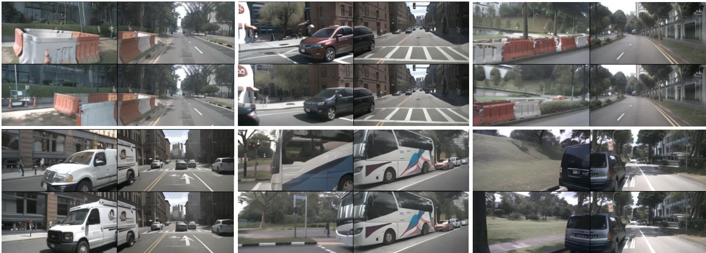
Figure 6. Qualitative results of factorized multiview generation. For each compared pair, the upper row is generated without factorization, and the lower row is generated with factorization.

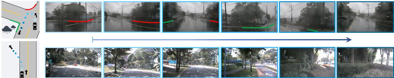
Figure 7. Counterfactual events generation. Top: turning around at a T-shape intersection on a rainy day. Note that our training set does not contain any turning-around samples. Bottom: running over a non-drivable area.

of using the ground truth driving command, we sample planned trajectories from VAD according to the three commands “Go straight”, “Turn left”, and “Turn right”. Then the sampled actions are used for our tree-based planning (Sec. 4). As shown in Table 3, our tree-based planner outperforms random driving commands and even achieves performance close to the GT command. Besides, in Table 4, we ablate two adopted rewards and the results indicate that the combined reward outperforms each sub-reward, particularly in terms of the object collision metric.

Table 5. Out-of-domain planning. We define OOD location with a lateral deviation of 0.5 meters from the ego vehicle.

	OOD World Model f.t.	L2(m)↓			Collision (%)↓
			2s3s	Avg.		1s2s3s		Avg.
		0.41 0.70 1.05			0.72	0.070.17 0.41		0.22
广		0.730.991.33			1.02	1.25 1.62 1.91		1.59
	√	0.50 0.79		1.17	0.82	0.72 0.84 1.16		0.91

Recovery from OOD ego deviation. Using our world model, we can simulate the out-of-domain ego locations in pixel space. In particular, we shift the ego location laterally by 0.5 meters, like the right one in Figure 2. In this situation, the performance of the existing end-to-end planner VAD [30] undergoes a significant decrease, shown in Table 5. To alleviate the problem, we fine-tune the planner with generated video supervised by the trajectory that the ego-vehicle drives back to the lane. Learning from these OOD data, the performance of the planner can be better and near normal levels.

5.5. Counterfactual Events

Given an initial observation and the action, our Drive-WM can generate counterfactual events, such as turning around and running over non-drivable areas (Figure 7), which are significantly different from the training data. The ability to generate such counterfactual data reveals again that our Drive-WM has the potential to foresee and handle out-ofdomain cases.

6. Conclusion

We introduce Drive-WM, the first multiview world model for autonomous driving. Our method exhibits the capability to generate high-quality and consistent multiview videos under diverse conditions, leveraging information from textual descriptors, layouts, or ego actions to control video 图6。分解多视角生成的定性结果。对于每组对比，上排为未使用因子分解生成，下排为使用因子分解生成。

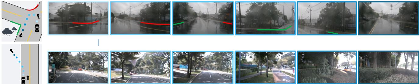
图 7。反事实事件生成。上：雨天在T型路口掉头。注意我们的训练集不包含任何掉头样本。下：驶入不可通行区域。

使用真实驾驶指令，我们根据“三条指令”“Gostraight”、“Turn left”和“Turn right”从VAD中采样规划轨迹。然后将采样到的动作用于我们的基于树的规划（第4节）。如表3所示，我们的基于树的规划器优于随机驾驶指令，甚至达到接近真实指令的性能。此外，在表4中，我们消融了两种采用的奖励，结果表明组合奖励优于各个子奖励，尤其是在物体碰撞指标方面。

OOD 世界模型f.t.	L2(米）← 1s2s3s	Avg.	碰撞率（%）← 1s2s3s
	0.410.701.05		.07 0.17 0.41 0.	Avg.
广	0.73 0.99 1.33		.25 1.62 1.91 1.5
	0.50 0.79 1.17(		.72 0.84 1.16 0.

表格 5. 域外规划。我们将与自车横向偏差为 0.5 米的位置定义为 OOD 位置。

从域外自车偏差的恢复。 利用我们的世界模型，我们可以在像素空间中模拟域外的自车位置。具体来说，我们将自车位置横向平移0.5米，就像图中向右的那个2。在此情形下，现有端到端规划器 VAD [30] 的性能显著下降，见表5。为缓解该问题，我们用由自车返回车道轨迹监督生成的视频对规划器进行了微调。从这些域外数据中学习后，规划器的性能可以得到改善并接近正常水平。

5.5. 反事实事件

给定初始观测和动作，我们的 Drive‑WM 可以生成反事实事件，例如掉头并驶入不可通行区域（图7），这些事件与训练数据显著不同。生成此类反事实数据的能力再次表明我们的 Drive‑WM 有预见并处理域外情况的潜力。

6. 结论

我们提出了 Drive‑WM，这是首个用于自动驾驶的多视角世界模型。我们的方法能够在多种条件下生成高质量且一致的多视角视频，并利用文本描述、布局或自车动作等信息来控制视频

generation. The introduced factorized generation significantly enhances spatial consistency across various views. Besides, extensive experiments on nuScenes dataset show that our method could enhance the overall soundness of planning and robustness in out-of-distribution situations.

生成。所引入的因子化生成显著增强了各视图间的空间一致性。此外，在 nuScenes 数据集上的大量实验证明，我们的方法能够提升规划的整体合理性，并在分布外情况下提高鲁棒性。

Driving into the Future: Multiview Visual Forecasting and Planning with World Model for Autonomous Driving

Supplementary Material

A. Qualitative Results

In this section, we present qualitative examples that demonstrate the performance of our model. For the full set of video results generated by our model, please see our anonymized project page at https://drive-wm.github.io.

A.1. Generation of Multiple Plausible Futures

Drive-WM can predict diverse future outcomes according to maneuvers from planners, as shown in Figure 8. Based on plans from VAD [30], Drive-WM forecasts multiple plausible futures consistent with the initial observation. We generate video samples on the nuScenes [5] validation set. The rows in Figure 8 show predicted futures for lane changes to left or keep the current lane (row 1), driving towards the roadside and straight ahead (row 2), and left/right turns at intersections (row 3).

A.2. Generation of Diverse Multiview Videos

Drive-WM can function as a multiview video generator conditioned on temporal layouts. This enables applications as a neural simulator for Drive-WM. Although trained on nuScenes [5] train set, Drive-WM exhibits creativity on the val set by generating novel combinations of objects, motions, and scenes.

Normal scenes generation. Drive-WM can generate diverse multiview video forecasts based on layout conditions, as shown for the nuScenes [5] validation set in Figure 9.

Rare scenes generation. It can also produce high-quality videos for rare driving conditions like nighttime and rain, despite limited exposure during training, as illustrated in Figure 10. This demonstrates the model’s ability to generalize effectively beyond the daytime scenarios dominant in the training data distribution.

A.3. Visual Element Control

Drive-WM allows conditional generation through various forms of control, including text prompts to modify global weather and lighting, ego-vehicle actions to change driving maneuvers, and 3D boxes to alter foreground layouts. This section demonstrates Drive-WM’s flexible control mechanisms for interactive video generation based on user-specified conditions.

Weather & Lighting change. As shown in Figure 11 and Figure 12, we demonstrate the ability of our model to change weather or lighting conditions while maintaining the same scene layout (road structure and foreground objects). Video examples are generated based on the layout conditions from nuScene val set. This ability has great potential for future data augmentation. By generating diverse scenes under various weather and lighting conditions, our model can significantly expand the training dataset, thereby improving the generalization performance and robustness of the model.

Action control. Our model is capable of generating highquality street views consistent with given ego-action signals. For instance, as shown in Fig. 14, our model correctly generates turning-left and turning-right videos from the same initial frame according to the input steering signals. In Fig. 15, our model successfully predicts the positions of the surrounding vehicles conforming with both the accelerating and decelerating signals. These qualitative results demonstrate the high controllability of our world model.

Foreground control. As Figure 13 shows, Drive-WM enables fine-grained control of foreground layouts in generated videos. By modifying lateral and longitudinal conditions, high-fidelity images are produced that correspond to the layout changes specified.

Pedestrian generation poses challenges for street-view synthesis methods. However, unlike previous work [53, 69], Figure 16 shows Drive-WM can effectively generate pedestrians. The first six images displays a vehicle waiting for pedestrians to cross, while the second six images shows pedestrians waiting at a bus stop. This demonstrates our model’s potential to produce detailed multi-agent interactions.

A.4. End-to-end Planning Results for Out-ofdomain Scenarios

Existing end-to-end planners are trained on expert trajectories aligned to lane centers. As Figure 2 shows, this causes difficulties generating off-center deviations, known as the “lack-of-exploration” problem in behavior cloning [8]. Using Drive-WM for simulation, Figure 18 demonstrates more planned trajectories deviating from the lane center. We find the planner from [30] cannot recover when evaluated on these generated out-of-distribution cases. This highlights

驶向未来：多视角视觉预测与基于世界模型的自动驾驶规划

补充材料

A. 定性结果

在本节中，我们展示了一些定性示例来说明我们模型的性能。有关我们模型生成的全部视频结果，请参见我们匿名的项目页面：https://drive-wm.github.io。

A.1. 生成多种合理未来

Drive‑WM 可以根据规划器的机动动作预测多样的未来结果，如图8所示。基于来自 VAD 的计划 [30], ，Drive‑WM 预测出与初始观测一致的多种合理未来。我们在nuScenes验证集上生成视频样本。图8 的行分别显示了对变道到左侧或保持当前车道（第 1 行）、向路边行驶和直行（第 2 行）、以及路口处左/右转（第 3 行）的预测未来。

A.2. 生成多样化多视角视频

Drive‑WM可以作为一个基于时序布局的多视角视频生成器运行。[5]尽管在nuScenes 训练集上训练，Drive‑WM在验证集上通过生成对象、运动和场景的新组合展现了创造性。

常规场景生成。 Drive‑WM能够基于布局条件生成多样的多视角视频预测，如图 [5]所示的 nuScenes 验证集在图9。

罕见场景生成。它也能为诸如夜间和降雨等罕见驾驶条件生成高质量视频，尽管在训练期间对此类情形接触有限，如图10所示。这表明模型能够有效地推广，超越训练数据分布中以白天场景为主的情形。

A.3. 视觉元素控制

Drive‑WM 支持通过多种控制形式进行条件生成，包括通过文本提示修改整体天气和光照、通过自车动作改变驾驶机动动作，以及通过 3D 立方体调整前景布局。本节展示了 Drive‑WM 基于用户指定条件进行交互式视频生成的灵活控制机制。

Weather & Lighting change. As shown inFigure11and Figure12，我们展示了模型在保持相同场景布局（道路结构和前景对象）的同时更改天气或光照条件的能力。视频示例基于 nuScene val 集的布局条件生成。这一能力对未来的数据增强具有巨大潜力。通过在各种天气和光照条件下生成多样化的场景，我们的模型可以显著扩展训练数据集，从而提高模型的泛化性能和鲁棒性。

动作控制。 我们的模型能够生成与给定自车动作信号一致的高质量街景视图。例如，如图14所示，模型能根据输入的转向信号从相同初始帧正确生成左转和右转的视频。在图15中，模型还能成功预测周围车辆的位置，分别符合加速和减速信号。这些定性结果展示了我们世界模型的高可控性。

前景控制。 如图 13所示，Drive‑WM 能够对生成视频中的前景布局进行细粒度控制。通过修改横向和纵向条件，能够生成与所指定布局变化相对应的高保真图像。

行人生成对街景合成方法提出了挑战。然而，与先前工作不同 [53, 69],图 16显示 Drive‑WM 可以有效生成行人。前六张图展示了一辆车在等待行人过马路，而后六张图展示了行人在公交站等待。这表明我们的模型有能力生成细致的多智能体交互。

A.4. 面向域外场景的端到端规划结果

现有的端到端规划器是在与车道中心对齐的专家轨迹上训练的。正如图2所示，这导致在生成偏离车道中心的行为时遇到困难，这在行为克隆中被称为“缺乏探索”问题 [8]。使用 Drive‑WMforsimulation，图18 展示了更多偏离车道中心的规划轨迹。我们发现来自 [30]的规划器在这些生成的分布外样例上评估时无法恢复。这凸显了

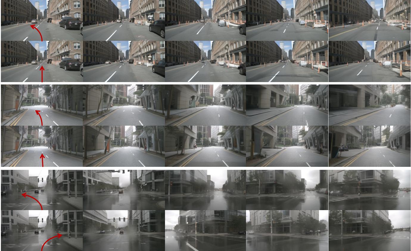
Figure 8. Generation of multiple plausible futures based on the planning. Here we only show the front-view videos for better illustration. The video samples are generated based on the first frames from the nuScenes val set. In the first row, we show examples of lane changing to the left and straight ahead. In the second row, we show cases of driving towards the roadside and driving straight ahead. In the last row, we present examples of making left and right turns at the intersection.

the utility of Drive-WM for exploring corner cases and improving robustness.

A.5. Using GPT-4V as a Reward Function

To assess the safety of different futures forecasted under different plans, we leverage the recent GPT-4V model as an evaluator. Specifically, we use Drive-WM to synthesize diverse future driving videos with varying road conditions and agent behaviors. We then employ GPT-4V to analyze these simulated videos and provide holistic rewards in terms of driving safety. As illustrated in Figure 17, it demonstrates different driving behaviors that GPT-4V plans when there is a puddle ahead on the road. Compared to reward functions with vectorized inputs, GPT-4V provides a more generalized understanding of hazardous situations in the Drive-WM videos. By deploying GPT-4V’s multimodal reasoning capacity for future scenario assessment, we enable enhanced evaluation that identifies risks not directly represented but inferred through broader scene understanding. This demonstrates the value of combining generative world models like Drive-WM with reward-generating models like GPT-4V. By using GPT-4V to critique Drive-WM’s forecasts, more robust feedback can be achieved to eventually improve autonomous driving safety under diverse realworld conditions.

A.6. Video Generation on Other Datasets

Waymo Open Dataset. To showcase the wide applicability of Drive-WM, we apply it to generate high-resolution $768\times 512$ images on the Waymo Open Dataset. As seen in Figure 19 and Figure 20, Drive-WM produces realistic and diverse driving forecasts at this resolution with the same hyper-parameters for nuScenes. By generalizing effectively to new datasets and resolutions, these Waymo examples verify that Drive-WM provides a widely adaptable approach to high-fidelity video synthesis across different driving datasets.

B. Implementation Details

In this section, we introduce the training & inference details of joint multiview video model and factorization model.

图8。基于规划生成多种合理未来。此处我们仅展示前视视频以更好地说明。视频样本基于 nuScenes val集的第一帧生成。第一行展示了变道到左侧和直行的示例。第二行展示了向路边行驶和直行的案例。最后一行展示了在路口左转和右转的示例。

Drive‑WM 在探索角落情况和提高鲁棒性方面的价值。

A.5. 使用 GPT‑4V 作为奖励函数

为了评估在不同策略下预测的不同未来情形的安全性，我们利用最新的 GPT‑4V 模型作为评估器。具体而言，我们使用 Drive‑WM 合成在不同道路条件和主体行为下的多样化未来驾驶视频。然后我们使用 GPT‑4V 分析这些模拟视频，并就驾驶安全性方面提供整体奖励。如图17 所示，它展示了当道路前方有水坑时 GPT‑4V 规划出的不同驾驶行为。与采用向量化输入的奖励函数相比，GPT‑4V 对 Drive‑WM 视频中危险情形提供了更通用的理解。通过利用 GPT‑4V 的多模态推理能力进行未来情景评估，我们实现了更强的评估能力，能够识别那些并未被直接表示但可通过更广泛场景理解推断出的风险。这证明了将像 Drive‑WM 这样的生成式世界模型与像GPT‑4V 这样的奖励生成模型相结合的价值。通过使用GPT‑4V 来批评 Drive‑WM 的

预测，可以获得更稳健的反馈，从而最终在多样的真实世界条件下提升自动驾驶安全性。

A.6. 在其他数据集上的视频生成

Waymo Open Dataset. 为展示 Drive‑WM 的广泛适用性，我们将其应用于在 $768\times 512$ Waymo OpenDataset 上生成高分辨率19和图 20中可见，Drive‑WM 在与 nuScenes 相同的超参数下，在此分辨率上生成了真实且多样的驾驶预测。通过有效地推广到新数据集和分辨率，这些 Waymo 示例验证了Drive‑WM 在不同驾驶数据集上提供一种对高保真视频合成广泛适应的方法。

B. 实施细节

在本节中，我们介绍joint multiview video model 和factorization model的训练与推理细节。

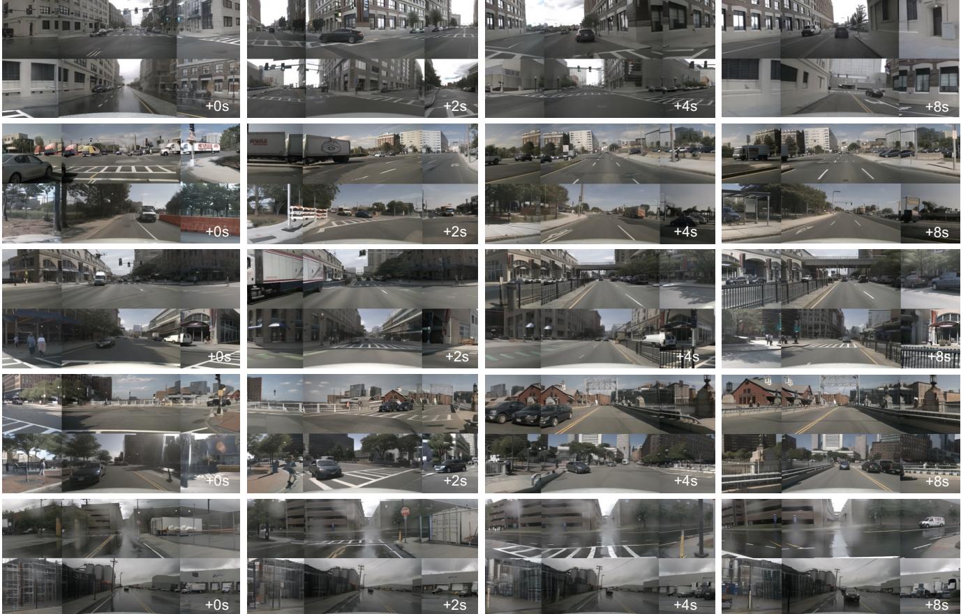
Figure 9. Conditional generation of diverse multiview videos. Given layout conditions (3D box, HD map, and BEV segmentation) from the nuScenes val set, our model is able to generate spatio-temporal consistent multiview videos.

B.1. Joint Multiview Video Model

Training Details. The original image resolution of nuScenes is $1600\times 900$ . We initially crop it to $1600\times$ 800 by discarding the top area and then resize it to $384\times$ 192 for model training. Similar to VideoLDM [2], we begin by training a conditional image latent diffusion model. The model is conditioned on various scene elements, such as HD maps, BEV segmentation, 3D bounding boxes, and text descriptions. All the conditions are concatenated in the token-length dimension. The image model is initialized with Stable Diffusion checkpoints [44] This conditional image model is trained for 60,000 iterations with a total batch size of 768. We use the AdamW optimizer with a learning rate $1\times 10^{-4}$ . Subsequently, we build the multiview video model by introducing temporal and multiview parameters (Sec. 3.1) and fine-tune this model for 40,000 iterations with a batch size of 32, with video frame length $T=8$ . For action-based video generation, the difference lies only in the change of condition information for each frame, while the rest of the training and model structure are the same. We use the AdamW optimizer [32] with a learning rate $5\times 10^{-5}$ for the video model. To sample from our models, we generally use the sampler from Denoising Diffusion Implicit Models (DDIM) [50]. Classifier-free guidance (CFG) reinforces the impact of conditional guidance. For each condition, we randomly drop it with a probability of $20\%$ during training. All experiments are conducted on A40 GPUs.

Inference Details. During inference, the number of sampling steps is 50, and we use stochasticity $\eta =1.0$ , $\mathrm{CFG}=5.0$ . For video generation, we use the first frame as the condition to generate subsequent video content. Similar to VideoLDM [2], we use the generated frame as the subsequent condition for long video generation.

B.2. Factorization Model

Training implementation of factorization. The implementation is overall similar to the implementation of the joint modeling in Sec. B.1. For the factorized generation, we additionally use reference views as extra image conditions.

Taking nuScenes data as an example, we first sort the six multiview video clips clockwise, denoted as

图9。多视角视频的条件生成与多样性。给定来自 nuScenes 验证集的布局条件（3D 立方体、高清地图和鸟瞰视图分割），我们的模型能够生成时空一致的多视角视频。

B.1. 联合多视角视频模型

训练细节。nuScenes 的原始图像分辨率为

$1600\times 900_{\circ }$ 。我们最初将其裁剪为 $1600\times 800$ ，去掉顶部区域，然后将其调整为 $384\times 192$ 用于模型训练。与 VideoLDM 类似 [2], ，我们首先训练一个条件图像潜在扩散模型。该模型以多种场景要素为条件，例如高清地图、鸟瞰视图分割、三维边界框 和 文本描述。所有条件在令牌长度维度上拼接。图像模型由Stable Diffusion 检查点初始化 [44] 该条件图像模型训练 60,000 次迭代，总批量大小为 768。我们使用AdamW 优化器，学习率为 $1\times 10^{-4}$ 。随后，我们通过引入时间和多视图参数（第multiview videomodel 参见第3.1节）构建多视图视频模型，并以批量大小 32对该模型进行微调 40,000 次迭代，视频帧长度为$T=8_{\circ }$ 。对于基于动作的视频生成，差异仅在于每帧条件信息的变化，其余训练与模型结构相同。我们使用 AdamW 优化器 [32]，学习率为 $5\times 10^{-5}$ 用于

视频模型。为了从我们的模型中采样，我们通常使用去噪扩散隐式模型（DDIM）的采样器 $[50{]}_{\circ }$ 。无分类器引导（CFG）强化了条件引导的影响。对于每个条件，我们在训练期间以 $20\%$ 的概率随机丢弃。所有实验均在 A40 GPU 上进行。

推理细节。 在推理过程中，采样步数为50，并且我们使用随机性 $\eta =1.0$ ， $\mathrm { C F G } = 5 . 0 $ 。对于视频生成，我们使用第一帧作为条件来生成后续视频内容。与VideoLDM [2], 类似，我们在长视频生成中将生成的帧用作后续的条件。

B.2. 因式分解模型

因式分解的训练实现。 该实现总体上与第B.1节中联合建模的实现相似。对于因子化生成，我们还额外使用参考视图作为额外的图像条件。

以 nuScenes 数据为例，我们首先按顺时针对六个多视角视频片段进行排序，记为

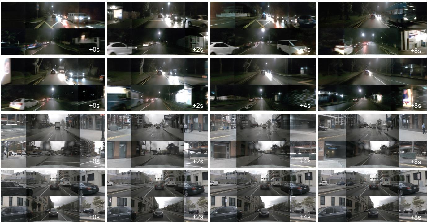
Figure 10. Rare scenes generation. Top two rows: night scenarios. Bottom two rows: rainy scenarios.

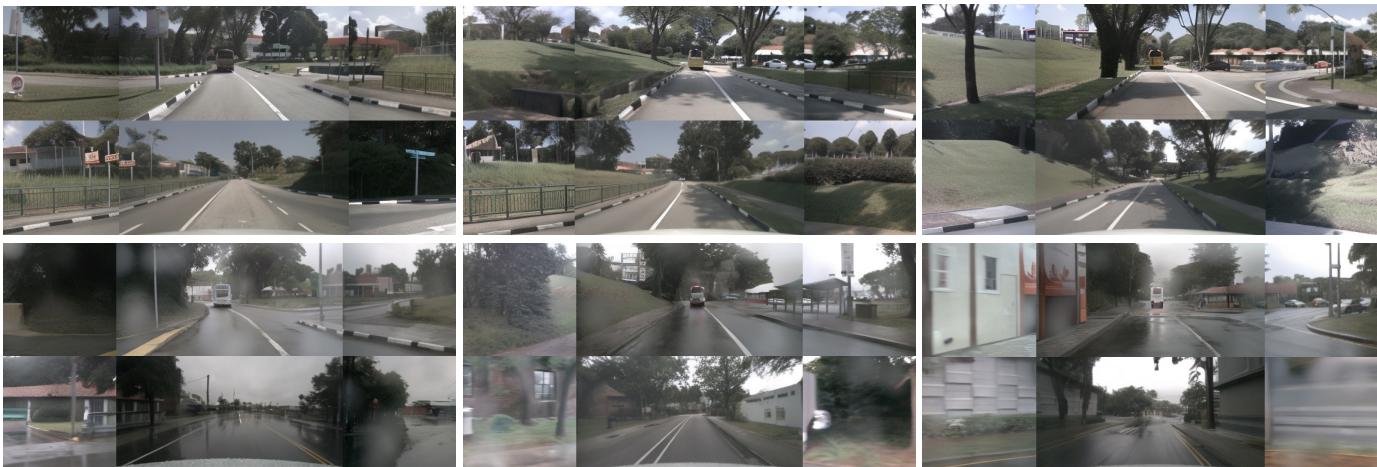
Figure 11. Weather change generation. The top row displays sunny daylight scenes. The bottom row shows the same layouts rendered as rainy scenes, demonstrating conditional generation capabilities.

${\mathbf{x}}_0$ to ${\mathbf{x}}_5$ . Then a training sample is defined as $\left\{{\mathbf{x}}_{(i-1)\mathrm{mod}6},{\mathbf{x}}_i,{\mathbf{x}}_i^{\prime },{\mathbf{x}}_{(i+1)\mathrm{mod}6}\right\}$ . where ${\mathbf{x}}_i$ is the stitched view randomly sampled from all six views, and {x(i−1)\{ \mathbf { x } _ { ( i - 1 ) }{x(i−1)​ mod ${}_6,{\mathbf{x}}_{(i+1)\mathrm{mod}6}\}$ is a pair of reference view. ${\mathbf{x}}_i^{\prime }$ is the previously generated frame of $i$ -th view, which also serves as an additional image condition. The training pipeline is very similar to the joint modeling, while here we generate a single view every iteration instead of multiple views. As can be seen from the training sample $\left\{{\mathbf{x}}_{(i-1)\mathrm{mod}6},{\mathbf{x}}_i,{\mathbf{x}}_i^{\prime },{\mathbf{x}}_{(i+1)\mathrm{mod}6}\right\}$ , we have view dimension $N=1$ for the single stitch view ${\mathbf{x}}_i$ in training.

Inference of factorization. During inference, we predefine some views as the reference views, and the corresponding videos of these reference views are first generated by the joint model. Then we generate the videos of stitched views conditioned on the paired reference video clips and previously generated view (i.e., ${\mathbf{x}}_i^{\prime },$ ). Particularly, in nuScenes, we select F, BL, $\mathtt{B}{\mathtt{R}}^3$ as reference views.

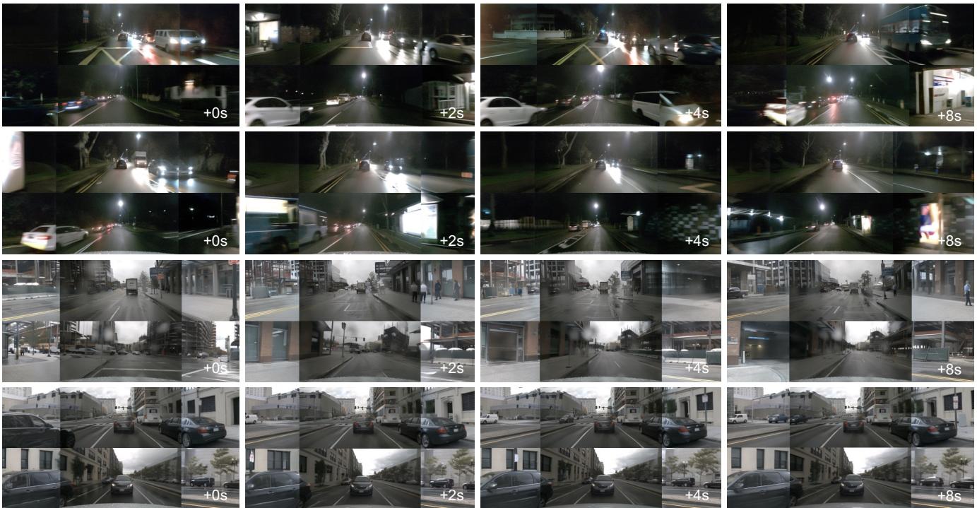
Figure 10. 稀有场景生成。上面两行：夜间场景。下面两行：雨天场景。

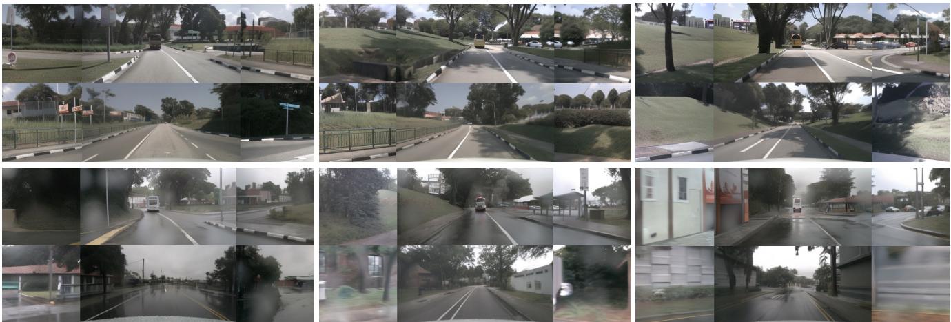
Figure 11. 天气变化生成。上排展示晴天白昼场景。下排显示相同布局渲染为雨天场景，展示了条件生成能力。

${\mathbf{x}}_0$ 到 ${\mathbf{x}}_{5\circ }$ 。然后一个训练样本被定义为 {x(i−1)\left\{ { \bf x } ( i - 1 ) \right.{x(i−1) mod 6，${\mathbf{x}}_i$ ， ${\mathbf{x}}_i^{\prime }$ ， $\mathbf{X}(i+1)\mathrm{mod}6{\}}_{(}$ 。其中 ${\mathbf{x}}_i$ 是从所有六个视图中随机采样的拼接视图， $\left\{{\mathbf{x}}_{(i-1)\mathrm{mod}6},{\mathbf{x}}_{(i+1)\mathrm{mod}6}\right\}$ 是一对参考视图。 ${\mathbf{x}}_i^{\prime }$ 是第 $i$ 个视图先前生成的帧，同时也作为额外的图像条件。训练流程与联合建模非常相似，但在此我们每次迭代只生成单个视图，而不是多个视图。正如从训练样本中可以看出 {x(i−1) mod 6\{ \mathbf { x } ( i - 1 ) { \bmod { 6 } }{x(i−1)mod6 ， ${\mathbf{x}}_i$ ， ${\mathbf{x}}_i^{\prime }$ ，$\mathbf{x}(i+1)\mathrm{mod}6\}$ ，我们具有视图维度‑

sion $N=1$ 用于单拼接视图 ${\mathbf{x}}_i$ 在训练中.

因式分解推断。在推断过程中，我们预先将若干视图定义为参考视图，这些参考视图对应的视频首先由联合模型生成。然后我们在配对参考视频片段和先前生成的视图（即 ${\mathbf{x}}_i^{\prime })$ ）的条件下生成拼接视图的视频。特别是在nuScenes 中，我们选择 F, BL, $\mathtt{B}{\mathtt{R}}^3$ 作为参考视图。

Figure 12. Lighting change generation. The top row displays daytime scenes. The bottom row shows the same layouts rendered as nighttime scenes, demonstrating conditional generation capabilities.

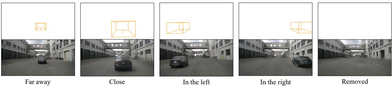
Figure 13. Control foreground object layouts. By modifying the positions of 3D boxes, high-fidelity images are produced that correspond to the layout changes specified.

The three reference views constitute three pairs, serving as the condition for three stitched views. For example, our model generates front-left views conditioning on front views, back-left views, and previously generated front-left views. The inference parameters are the same with Sec. B.1.

C. Data

In this section, we first describe the dataset preparation and then introduce the curation of the dataset to enhance the action-based generation.

C.1. Data Preparation

NuScenes Dataset. The nuScenes dataset provides full 360-degree camera coverage and is currently a primary dataset for 3D perception and planning. Following the official configuration, we use 700 street-view scenes for training and 150 for validation. Next, we introduce the processing of each condition. For the 3D box condition, we project the 3D bounding box onto the image plane, utilizing octagonal corner points to depict the object’s position and dimensions, while colors are employed to distinguish different categories. This ensures accurate object localization and discrimination between different objects. For the HD map condition, we project the vector lines onto the image plane, with colors indicating various types. In terms of the BEV segmentation, we adhere to the generation process outlined in CVT [72]. This process generates a bird’s-eye view segmentation mask, which represents the distribution of different objects and scenery in the scene. For the text condition, we sift through information provided in each scene description. For the planning condition, we utilize the ground truth movement of the ego locations for training, and the planned output from VAD [30] for inference. This allows the model to learn from accurate ego-motion information and make predictions that are consistent with the planned trajectory. Finally, for the ego-action condition, we extracted the information of vehicle speed and steering for each frame.

The Waymo Open Dataset. The Waymo Open Dataset [52] is a well-known large-scale dataset for autonomous driving. We only utilize data from the ”front” camera to train the video model, with an image resolution of $768\times 512$ pixels. For the map condition, we follow the data processing in OpenLane [7].

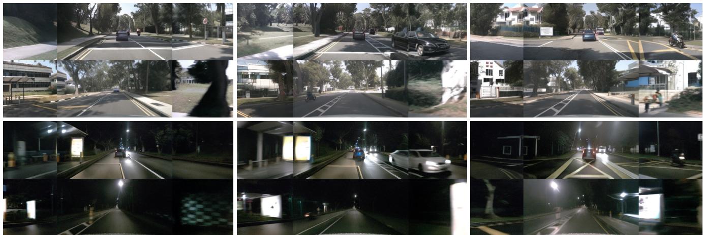
图12。光照变化生成。顶排展示白天场景。底排展示相同布局渲染为夜间场景，演示了条件生成能力。

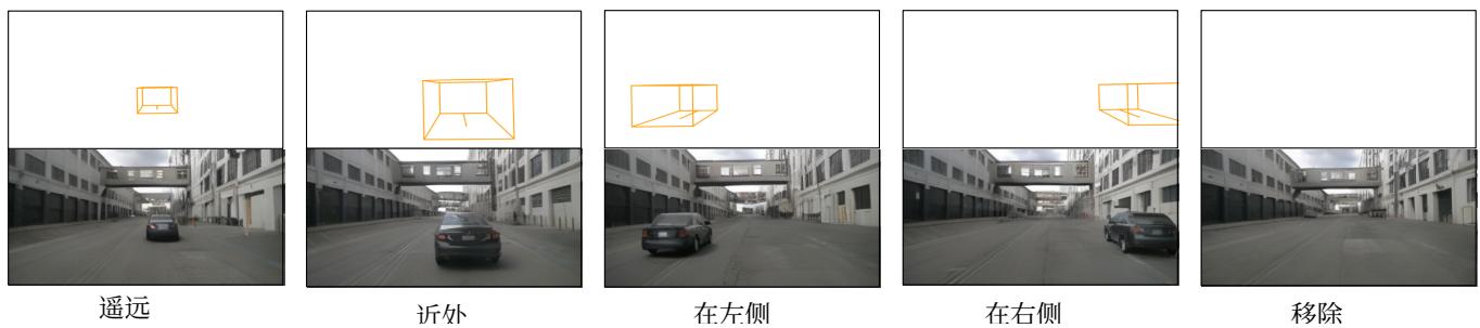
图13。控制前景对象布局。通过修改3D 立方体的位置，可以生成与所指定布局变化相对应的高保真图像。

这三个参考视图构成三对，作为三个拼接视图的条件。例如，我们的模型在以前视图、后左视图和先前生成的前左视图为条件的情况下生成前左视图。推理参数与第 B.1 节相同。

C. 数据

在本节中，我们首先描述数据集的准备工作，然后介绍为增强基于动作的生成而进行的数据集整理。

C.1. 数据准备

NuScenesDataset. nuScenes 数据集提供完整的 360度相机覆盖，目前是三维感知和规划的主要数据集。按照官方配置，我们使用 700 个街景场景作为训练集，150 个作为验证集。接下来介绍每种条件的处理流程。对于 3D 盒条件，我们将三维边界框投影到图像平面，利用八角角点来描述对象的位置和尺寸，并使用颜色来区分不同类别。这可确保准确的对象定位和

对象之间的区分。对于高清地图条件，我们将矢量线投影到图像平面，使用颜色表示不同类型。在鸟瞰视图分割方面，我们遵循 CVT 中描述的生成流程 $[72{]}_{\circ }$ 该流程生成一个鸟瞰视图分割掩码，表示场景中不同对象和景物的分布。对于文本条件，我们从每个场景描述中筛选信息。对于规划条件，训练时我们使用自车位置的真实运动，推理时使用 VAD 的规划输出 $[30{]}_{\circ }$ 这使模型能够从准确的自车运动信息中学习，并生成与规划轨迹一致的预测。最后，对于自车动作条件，我们提取了每帧的车辆速度和转向信息。

Waymo Open 数据集。Waymo Open 数据集 [52]是一个著名的大规模自动驾驶数据集。我们仅使用“前方”摄像头的数据来训练视频模型，图像分辨率为 $768\times 512$ 像素。关于地图条件，我们遵循OpenLane [7]中的数据处理方式。

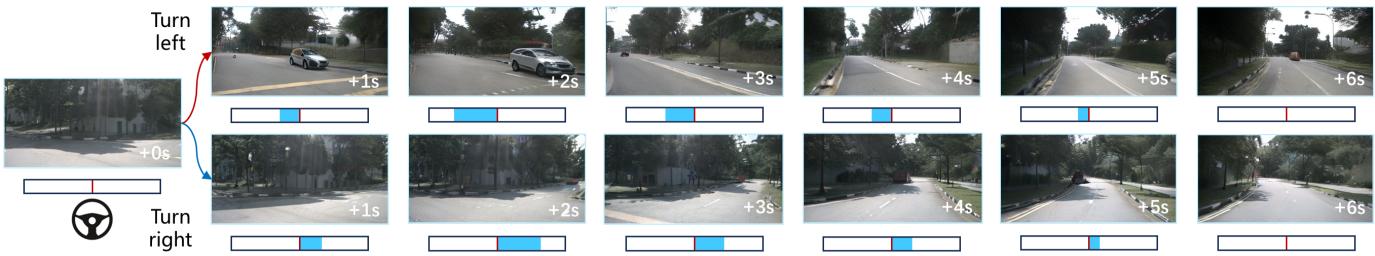
Figure 14. Diverse turning behaviors. Utilizing an identical initial frame, we provide our model with sequences of positive steering angles (indicating a left turn) and negative values (indicating a right turn). The figure demonstrates the model’s proficiency in generating consistent street views for both turning behaviors. Each frame is accompanied by a blue bar, indicating the corresponding steering angle in degrees. A longer bar correlates with a more substantial steering angle. For clarity, only the front view is shown.

Figure 15. Diverse speeding behaviors. We input different patterns of speed signals into our model to assess controllability in terms of speed. The top series shows that the ego car decelerates and then accelerates while the bottom one shows a contrary behavior. These two results highlight the realism of our model’s prediction.

C.2. Data Curation

The ego action distribution of the nuScenes dataset is heavily imbalanced: a large proportion of its frames exhibit small steering angles (less than 30 degrees) and a normal speed in the range of $10-20m/s$ . This imbalance leads to weak generalizability to rare combinations of steering angles and speeds.

To alleviate this negative impact, we balance our training dataset by re-sampling rare ego actions. Firstly, we split each trajectory into several clips, each of which demonstrates only one type of driving behavior (i.e., turning left, going straight, or turning right). This process results in 1048 unique clips. Afterward, we cluster these clips by digitizing the combination of average steering angles and speeds. The speed range [0, 40] $(m/s)$ is divided into 10 bins with equal lengths. Extreme speeds greater than $40m/s$ will fall into the 11th bin. The steering angle range [-150, 150] (degree) is divided into 30 bins with equal lengths. Likewise, extreme angles greater than 150 degrees or less than -150 degrees will fall into another two bins, respectively. We plot the ego-action distribution resulting from this categorization in Fig. 21.

To balance the action distribution of these clips, we sample $N=36$ clips from each bin of the 2D $32\times 11$ grid. For a bin containing more than $N$ clips, we randomly sample

$N$ clips; For a bin containing fewer than $N$ clips, we loop through these clips until $N$ samples are collected. Consequently, 7272 clips are collected. The action distribution after re-sampling can be seen in Fig. 21.

D. Metric Evaluation Details

D.1. Video Quality

The FID and FVD calculations are performed on 150 validation video clips from the nuScenes dataset. Since our model can generate multiview video, we break it down into six views of video for evaluation. We have a total of 900 video segments ( 40 frames) and follow the calculation process described in VideoLDM [2]. We use the official UCF FVD evaluation code4.

D.2. KPM Illustration

As mentioned in Sec. 5.1, we introduced the KPM score metric for measuring multiview consistency for generated images, which are not considered in both FID and FVD metrics. As shown in Figure 22, we demonstrate the keypoint matching process. The blue points are the keypoints in the overlapping regions on the left/right side of the image.

图14。多样的转弯行为。使用相同的初始帧，我们向模型提供正转向角序列（表示左转）和负值序列（表示右转）。图中展示了模型在生成两种转弯行为下保持一致街景视图的能力。每帧配有一条蓝色条，表示对应的转向角（度）。条越长表示转向角越大。为清晰起见，仅显示前视图。

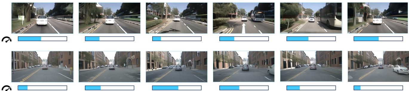
图15。多样的加速行为。我们向模型输入不同模式的速度信号，以评估在速度方面的可控性。上方序列显示自车先减速然后加速，而下方则表现出相反的行为。这两个结果突显了模型预测的逼真性。

C.2. 数据整理

nuScenes 数据集的自车动作分布高度不平衡：大量帧表现为较小的转向角（小于 30 度）且车速多在10‑20 米每秒的正常范围内。这种不平衡导致对罕见转向角与车速组合的泛化能力较弱。

为减轻这一负面影响，我们通过对稀有自车动作进行重采样来平衡训练集。首先，我们将每条轨迹切分为若干片段，每个片段仅展示一种驾驶行为（即左转、直行或右转）。此过程产生了1048 个唯一片段。随后，我们通过将平均转向角与速度的组合离散化来对这些片段进行聚类。速度范围 [0, 40] $(m/s)$ 被等长划分为10个区间。大于 $40\mathrm{m}/\mathrm{s}$ 的极端速度将落入第11个区间。转向角范围 [-150, 150] (度) 被等长划分为30个区间。同样地，大于150度或小于‑150度的极端角度将分别落入另外两个区间。我们在图21中绘制了由此分类得到的自车行为分布。

为了平衡这些片段的动作分布，我们从二维 $32\times 11$ 网格的每个箱中抽样 $N=36$ 个片段。对于包含超过 $N$ 个片段的箱，我们随机抽样

$N$ 片段；对于包含少于 $N$ 片段的箱子，我们循环这些片段直到 $N$ 个样本被收集为止。因此，共收集了7272 个片段。重采样后的动作分布如图 21 所示。

D. 指标评估细节

D.1. 视频质量

FID 和 FVD 的计算在 nuScenes 数据集中 150 个验证视频片段上进行。由于我们的模型可以生成多视图视频，我们将其拆分为六个视图的视频进行评估。我们共有900 段视频（40 帧），并遵循 VideoLDM 中描述的计算流程 [2]。我们使用官方的 UCF FVD 评估代码4。

D.2. KPM 说明

如第5.1节所述，我们提出了用于衡量生成图像多视角一致性的 KPM 分数度量，而该项并未被 FID 和FVD 指标所考虑。如图 22所示，我们展示了关键点匹配过程。蓝点是图像左右侧重叠区域中的关键点。

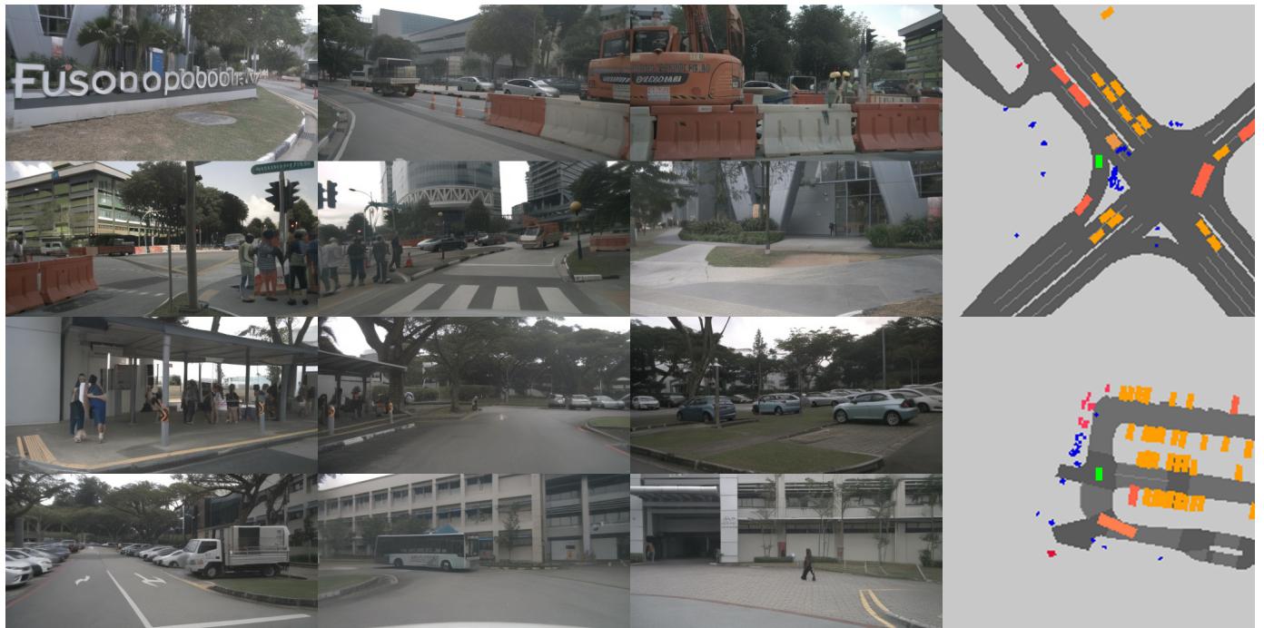
Figure 16. Pedestrian generation examples.

Describe the road surface condition first, please provide potential driving behaviors and the corresponding rewards.

The image depicts an overcast day with wet road conditions. There are areas of standing water on the road.

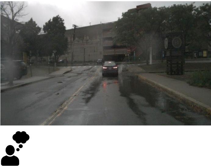
Figure 17. GPT-4V as a reward function. GPT-4V could give more reasonable rewards in cases such as there is a puddle ahead on the road.

• Avoiding Puddles: Steering around large puddles. Reward: Positive.
• Driving Through Puddles: If unavoidable, slowing down before entering the puddle to reduce the risk. Reward: Positive; However, if done at high speed, it could lead to loss of control. Reward: Negative.

The green lines are the matched points between the current view and its two adjacent views using the LoFTR [51] matching algorithm.

图16。 行人生成示例。

Describe the road surface condition first， please provide potential driving behaviors and the corresponding rewards.

The image depicts an overcast day with wet road conditions. There are areas of standing water on the road.

• Avoiding Puddles: Steering around large puddles. Reward: Positive.
• Driving Through Puddles: If unavoidable, slowing down before entering the puddle to reduce the risk. Reward: Positive; However, if done at high speed, it could lead to loss of control. Reward: Negative.

Figure 17. GPT‑4V 作为奖励函数。 在例如道路前方有水坑的情况下，GPT‑4V 可以给出更合理的奖励。

绿色线条表示当前视图与其两个相邻视图之间使用LoFTR [51]匹配算法的匹配点。

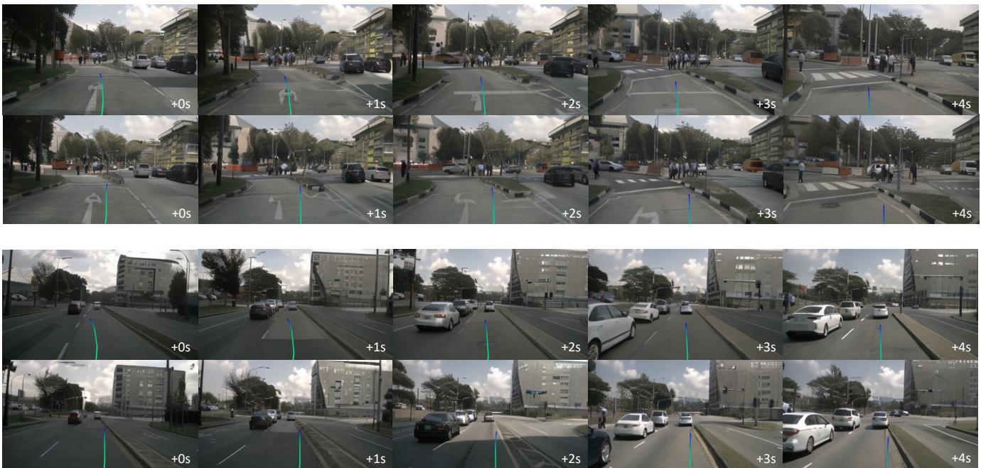
Figure 18. Videos demonstrating the VAD planning results under normal and out-of-domain cases. We shift the ego location $0.5\mathrm{m}$ to the right to create an out-of-domain case. The top row of each scene: the reasonable trajectory prediction of the VAD method under normal data. The bottom row of each scene: the irrational trajectory when encountering out-of-distribution cases.

Figure 19. Generation of High-Resolution Image on Waymo Open Dataset. We showcase the image generation results for a wide range of traffic density, driving scenarios, lighting, and weather conditions.

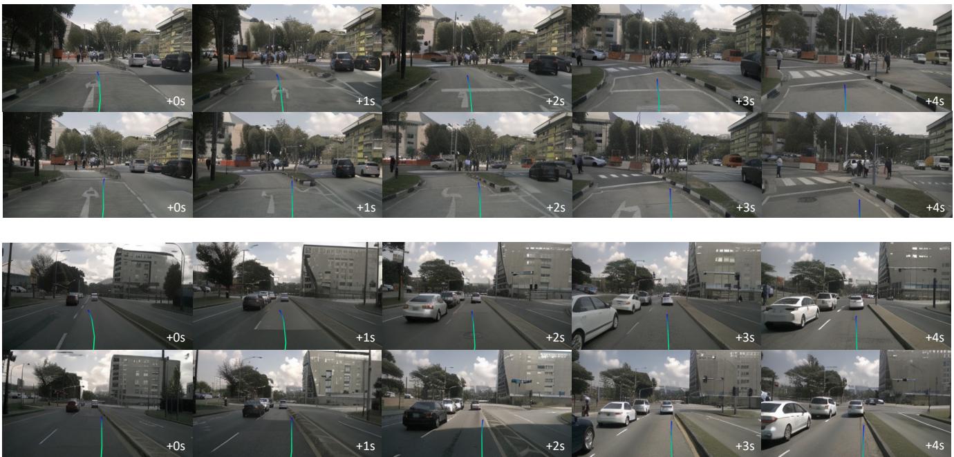
图18。展示在正常与域外情况下VAD 规划结果的视频。我们将自车位置向右平移 0.5 米以制造一个域外样例。每个场景的顶部行：VAD 方法在正常数据下合理的轨迹预测。每个场景的底部行：在遇到分布外样例时产生的不合理轨迹。

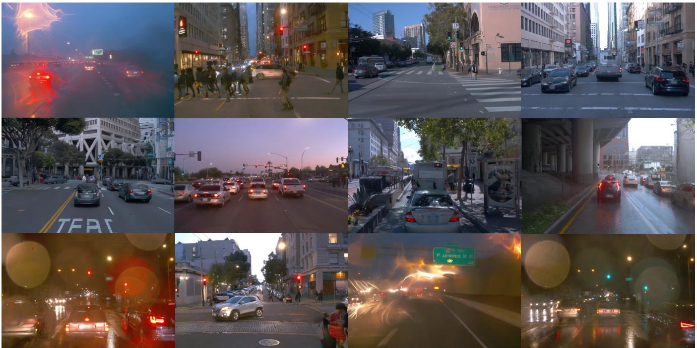
图19。在Waymo Open Dataset 上生成高分辨率图像。我们展示了在各种交通密度、驾驶场景、光照和天气条件下的图像生成结果。

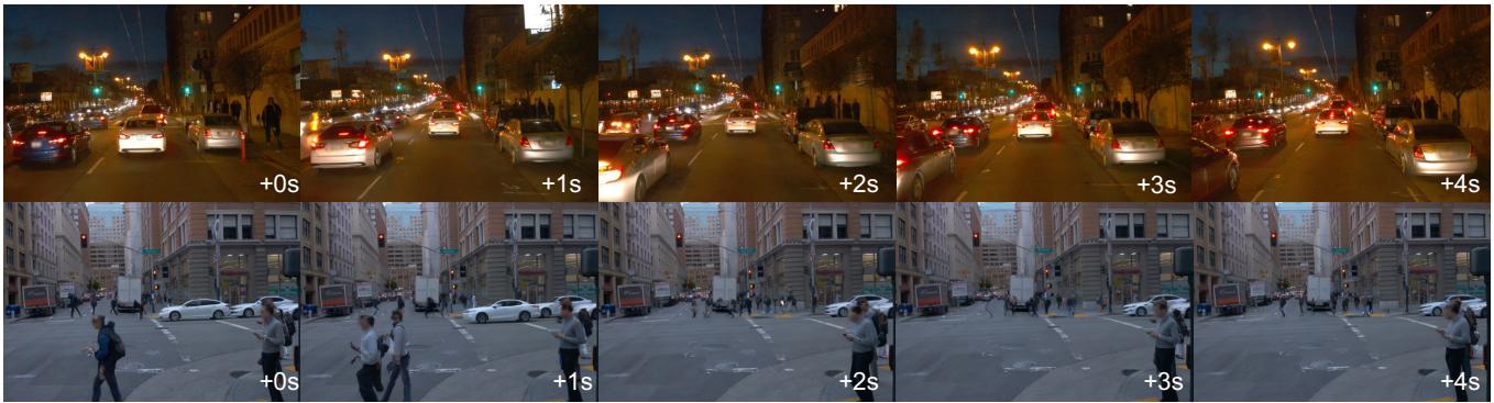
Figure 20. Generation of High-Resolution Video on Waymo Open Dataset. We showcase the video generation results in highly interactive driving scenarios like closely following the front car in heavy traffic (top) or waiting for pedestrians to cross the road.

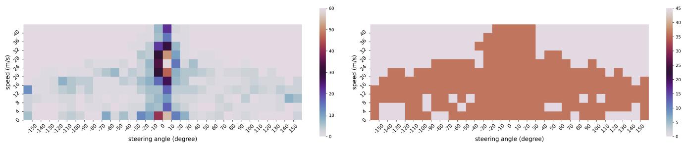
Figure 21. The ego-action distribution before (left) and after re-sampling (right). We re-sample rare combinations of speeds and steering angles, obtaining a balanced training dataset.

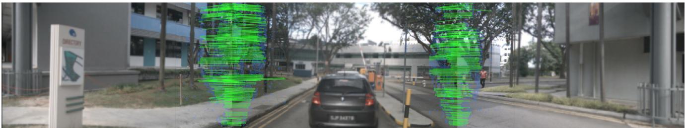
Figure 22. Illustration of keypoint matching in KPM calculation. The blue points are the image keypoints in the overlapping regions on the left/right side of the image. The green lines are the matched keypoints between the current view and its two adjacent views using the LoFTR [51] matching algorithm.

图 $20_{\circ }$ 。在Waymo Open Dataset 上生成高分辨率视频。我们展示了在高度交互的驾驶场景中的视频生成结果，例如在拥堵交通中紧随前车（上方）或等待行人过马路。

图 21。重采样前（左）和重采样后（右）的自车行为分布。我们对速度和转向角的稀有组合进行重采样，从而获得了平衡的训练数据集。

图22。 KPM 计算中关键点匹配的示意图。蓝色点表示图像左右侧重叠区域中的图像关键点。绿色线表示使用 LoFTR 在当前视图与其两个相邻视图之间匹配的关键点 [51] 匹配算法。