1. 背景

LTR, Learning-To-Rank, 对一组候选元素作 排序, 将序列(排列)视为一个整体, 追求 nDCG, MAP 等指标的提升. app 中的搜推场景就与 LTR 任务相匹配.

1.1 发展阶段

LTR 工作的发展分为几个阶段:

1. 早期阶段. 学习一个打分表达式中的参数. 如式 (1) 中的三个 w, 现已不是主流.
   $$score=w_1\cdot price+w_2\cdot ctr+w_3\cdot cvr\text{\hspace{1em}(1)}$$
2. 现代阶段. 使用 DNN 建模, 通过设计 loss 来优化排序效果. 又可分为 point-wise -> pair-wise -> list-wise 多个阶段. 整体属于 List-wise Training + Pointwise Inference 范式. 代表工作是 listNet.
3. 升级阶段, infer 阶段生成式预测 next-best 元素. 代表工作是 seq2Slate.

可列出表格作比较: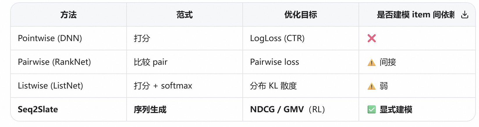

1.2 一些思考

Q1: List-wise Training + Pointwise Inference 范式中, 只是 train 阶段的 loss 用上了 list-wise, infer 方式仍是 point wise, 可为什么仍有效, 比纯 pointwise 方法要好?
A: 它改变了训练目标, 在 ListNet 的训练中，所有 item 的打分通过 softmax 归一化，形成“零和竞争”：模型被迫在一组候选内部做权衡，而不是孤立打分.
既然是实验科学, 实验证明 ListNet 的 NDCG 显著优于 RankNet（Pairwise）和 Regression（Pointwise）。

Q2: LTR 与 ctr预估 的关系?
A: LTR 是任务目标, ctr预估是实现路径之一.

2. 论文介绍

2.1 ListNet, ICML 2007

Listwise Learning to Rank 方法的奠基性工作. 论文名 Learning to Rank: From Pairwise Approach to Listwise Approach, 作者是 微软亚洲研究院.
首次系统提出 Listwise LTR 范式，并给出具体算法 ListNet. 在 LETOR 数据集上，ListNet 显著优于 RankSVM、RankBoost 等 Pairwise 方法.

思想

定义“理想排序”的概率分布（基于标签，如 NDCG 权重）
定义模型输出的排序概率分布（基于打分的 softmax）
用 交叉熵（Cross-Entropy） 或 KL 散度 作为 Loss.

loss 推导见附录.

实验

• 数据集, 其中一个是CSearch, 来自商业搜索引擎. This data set provides five levels of relevance judgments, ranging from 4 (”perfect match”) to 0 (”bad match”).
• 指标,nDCG@5 and MAP(mean average precision).

2.2 兼顾排序与概率准度(参考3论文)

YouTube 的工业实践.
list-wise 方法可以提升排序指标, 但会损失 score 的准度, 如 预估ctr 与实际ctr 偏差大, 该论文工作可 兼顾二者.

2.3 S-IE

该论文见参考[1].

Session Infomation Embedding (S-IE)

算是一个预训练, task为正负样本二分类, 为后面list-wise作准备.

图: 将点击与曝光内容分别pooling, 后与 target,user 作concat.

list-wise ranking

图 公式书写太差, 有误, (1)式中分子下标i可能为$t$,分母下标i可能为$l$; (2)式中i及右括号应放在上标位置.

实验

• 数据集. CIKM CUP 2016.是电商网站搜索引擎的日志.
• ndcg作指标. ctr预估, 通常用二分类的任务去做, 其指标为AUC/GAUC. 现在是list-wise, 就用nDCG.

我的疑惑

1. session s 的rep由target得到,即 $rep(session)=f(target,other)$ 那么 target 与 图2中的 n 个item是什么关系? 论文有说each session with the contained item behaviors is treated as a list-wisw training sample,但还不是很清楚.
2. 为啥用搜索引擎的日志, 找个推荐数据集不是更直接么?

2.4 Seq2Slate, Google 2018

Google 2018 年的工作, 论文见参考[4]. 它将排序问题建模为 “从候选集中依次选择 item 构建排序列表” 的序列生成任务，并采用 强化学习（RL） 或 策略梯度 进行端到端优化。
它代表了 LTR（Learning to Rank）从 “打分+排序” 范式 向 “生成式排序” 范式 的重要演进。
“a slate of” 是 “一系列, 一套 …” 的意思.

思考讨论

• 所谓 list-wise
  所谓list-wise 也只是损失函数相关, 预测阶段依旧是point-wise打分并排序, 由此得到序列.
  谷歌的Seq2Slate的论文里有一段清晰的描述：

In listwise approaches the loss depends on the full permutation of items. Although these losses consider inter-item dependencies, the ranking function itself is pointwise, so at inference time the model still assigns a score to each item which does not depend on scores of other items (i.e., an item’s score will not change if it is placed in a different set).

• loss 与 常规多分类 有何异同
  已经很像了, recsys中召回任务的设计就可以是transformer那样的多分类. 但常规的label是one-hot(可能带有 label smooth), 此处是一个不那么陡峭的分布.

附录

listwise loss 推导

论文1的list-wise借鉴了参考2, ICML’2017的微软的论文.
定义 list-wise 的损失函数:
$$\sum _{i=1}^{m}L(y^{(i)},z^{(i)})\text{\hspace{1em}(1)}$$
where $m=|trainset|$ , $y^{(i)}=(y_1^{(i)},y_2^{(i)},...,y_{n^{(i)}}^{(i)})$, 是一个list,表示与query $q^{(i)}$ 相关的 $n^{(i)}$ 个文档的相关性得分. 与之类似, $z^{(i)}=(f(x_1^{(i)}),f(x_2^{(i)}),...,f(x_{n^{(i)}}^{(i)}))$ 是 ranking function $f(\cdot )$ 计算出的预估相关性.

probability model

图: permutation probability
对size=n的list作全排列, 有 $n!$ 种结果, 计算量不可接受, 也就是 NP_Hard? 所以提出 top one probability.

图: top one probability.

图: 定理6, doc j 排第一的概率描述

图: 对$\varphi (\cdot )$作指数函数定义后, 可以改写 定理6 , 就成了soft-max

图: soft_max 得到 label与pred两个list的概率后, 用交叉熵作损失函数, 得到了最终的loss.

参考

1. ICML '2007, MIcrosoft, Learning to Rank: From Pairwise Approach to Listwise Approach
2. CIKM '2017, Alibaba, Session-aware Information Embedding for E-commerce Product Recommendation
3. CIKM '2023, Regression Compatible Listwise Objectives for Calibrated Ranking with Binary Relevance
4. 2018, Google, Seq2Slate: Re-ranking and Slate Optimization with RNNs