AI之模型提升
模型提升
目录
1.权重衰减
2.暂退法(Dropout)
3.优化算法
4.实战
概要
本文介绍了三种提升模型性能的关键技术:
- 权重衰减:通过 L2 正则化限制模型权重参数大小,在损失函数中加入权重平方项,使参数更新时被 “衰减”,从而防止过拟合。
- 暂退法(Dropout):训练时随机丢弃部分神经元,以类似集成学习的方式减少模型对单一特征的依赖;测试时保留所有神经元并缩放输出以保持输出期望一致,以此防止过拟合。
- 优化算法:
- 动量优化通过累积之前的更新方向形成 “惯性”,解决普通梯度下降的震荡和局部最优问题,加速收敛;
- Adam 算法结合动量(一阶矩)和自适应学习率(二阶矩),通过偏差修正解决初始阶段 “冷启动” 问题,优化参数更新过程。
一、权重衰减
权重衰减(Weight Decay) 是一种防止过拟合的技术,本质是让模型的权重参数尽可能小。
- 模型的权重就像人脑中的 “记忆强度”,权重越大,模型越容易记住复杂的细节(包括噪声);
- 权重衰减就像 “强制减肥”,让模型的 “记忆强度” 降低,从而忽略无关细节,抓住本质规律(比如学会解题方法而不是死记答案)。
原理:限制模型参数的大小,减少过拟合风险。
L2正则化
L2 正则化是深度学习中解决过拟合的核心技术之一
公式:
L′(θ)=L(θ)+λ2∑w∈θw2L'(\theta) = L(\theta) + \frac{\lambda}{2} \sum_{w \in \theta} w^2L′(θ)=L(θ)+2λw∈θ∑w2
梯度下降中的参数更新:为什么参数会“变小”?
训练时用梯度下降更新参数w,原始更新公式:
w←w−η⋅∂L(θ)∂ww \leftarrow w - \eta \cdot \frac{\partial L(\theta)}{\partial w}w←w−η⋅∂w∂L(θ)
加入L2正则化后,损失函数对w的梯度多了一项:
∂L′(θ)∂w=∂L(θ)∂w+λnw\frac{\partial L'(\theta)}{\partial w} = \frac{\partial L(\theta)}{\partial w} + \frac{\lambda}{n} w∂w∂L′(θ)=∂w∂L(θ)+nλw
二、暂退法(Dropout)
根据- 奥卡姆剃刀原理:更简单的模型(参数更小)可能会更好,也就是经典泛化理论认为,为了缩小训练和测试性能之间的差距,应该以简单的模型为目标。
而简单性的另一个角度是平滑性,即函数不应该对其输入的微小变化敏感。
1995年,克里斯托弗·毕晓普证明了 具有输入噪声的训练等价于Tikhonov正则化 (Bishop, 1995)。 这项工作用数学证实了“要求函数光滑”和“要求函数对输入的随机噪声具有适应性”之间的联系。
然后在2014年,斯里瓦斯塔瓦等人 (Srivastava et al., 2014) 就如何将毕晓普的想法应用于网络的内部层提出了一个想法: 在训练过程中,他们建议在计算后续层之前向网络的每一层注入噪声。 因为当训练一个有多层的深层网络时,注入噪声只会在输入-输出映射上增强平滑性。
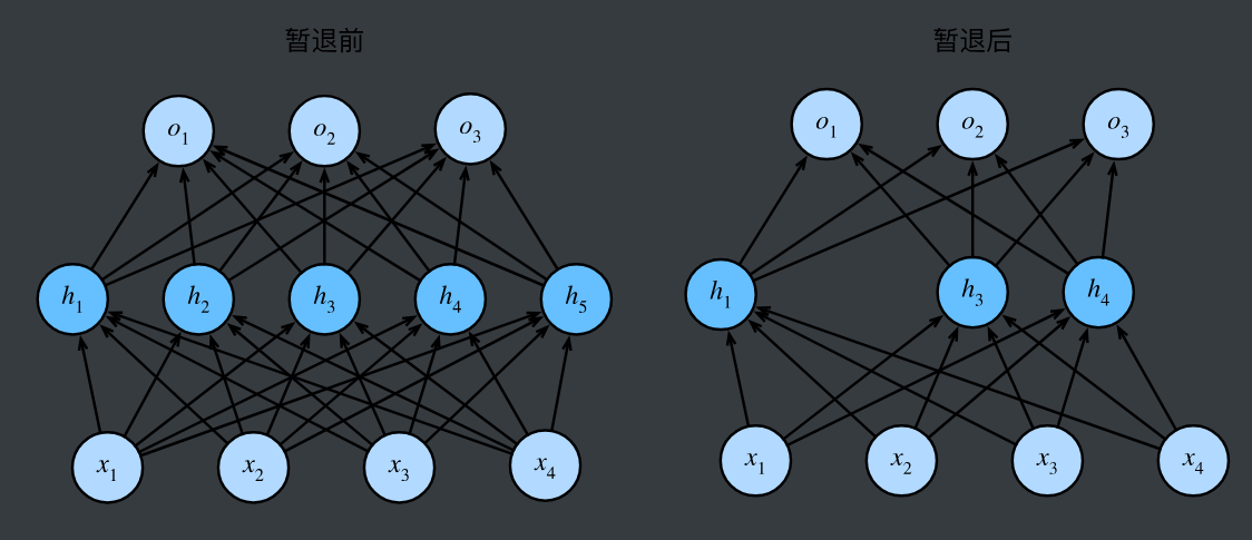
这个想法被称为暂退法(dropout)。 暂退法在前向传播过程中,计算每一内部层的同时注入噪声,这已经成为训练神经网络的常用技术。 这种方法之所以被称为暂退法,因为我们从表面上看是在训练过程中丢弃(drop out)一些神经元。 在整个训练过程的每一次迭代中,标准暂退法包括在计算下一层之前将当前层中的一些节点置零。
原理:在训练过程中,随机“忘记”一些神经元,每次更新时只使用一部分神经元,避免过拟合。
核心原理
- 训练阶段:随机“断电”神经元
- 对神经网络中的每个神经元,以概率p保留其输出,以概率1-p设为0(即“丢弃”)。
- 例如,若p=0.5,则每次训练时,每个神经元有50%的概率工作,50%的概率“休息”。
- 效果:每次训练相当于用一个“精简版”子网络学习,类似多个模型集成(集成学习),减少对单一特征的依赖。
- 测试阶段:保留所有神经元,但“缩放”输出
- 测试时需要使用完整网络,但为了和训练阶段的输出期望一致,需要将每个神经元的输出乘以 p(或训练时除以 p)。
- 例如,训练时神经元以 p 的概率输出x,期望为 $p \cdot x $;测试时乘以 p 后,期望变为 $ p \cdot x $,保持一致。
y=Dropout(x,p)=m⊙xy = \text{Dropout}(x, p) = m \odot xy=Dropout(x,p)=m⊙x
三、优化算法
动量优化(Momentum)
一、为什么需要动量?—— 普通梯度下降的 “绊脚石”
假设你在下山(寻找损失函数最小值),普通梯度下降(SGD)就像每次只看眼前一步的方向(当前梯度),走一步算一步:
问题 1:震荡徘徊:如果山路崎岖(梯度方向变化大),你会左右摇摆,浪费精力(收敛慢);
问题 2:陷入洼地:遇到小坑(局部最小值)就以为到了山脚,停止前进(易困局部最优)。
动量的核心思路:像滚石下山一样,利用 “惯性” 累积之前的运动方向,让下山更顺滑、更快。
二、动量优化的物理直觉:惯性累积与方向平滑
物理类比:滚石的动量
石头从山上滚下时,速度(方向和大小)不仅取决于当前坡度(当前梯度),还受之前滚动方向的影响(惯性);
坡度陡(梯度大)时,速度增加快;坡度缓(梯度小)时,惯性让石头继续滚动,避免停滞。
神经网络中的动量
每次参数更新时,不仅考虑当前梯度,还 “记住” 之前的更新方向,形成 “累积速度”;
梯度方向一致时,速度叠加,加速收敛;梯度方向变化时,惯性抵消部分震荡,平滑更新路径。
数学公式
三、 基础动量更新公式
设参数为 θ\thetaθ,学习率为 η\etaη,动量系数为 β\betaβ(通常0.9),梯度为 gtg_tgt,则:
- 速度更新:vt=β⋅vt−1+η⋅gtv_t = \beta \cdot v_{t-1} + \eta \cdot g_tvt=β⋅vt−1+η⋅gt
- 参数更新:θt=θt−1−vt\theta_t = \theta_{t-1} - v_tθt=θt−1−vt
Adam(Adaptive Moment Estimation)
原理:结合了动量优化和自适应学习率。
公式:
mt=β1mt−1+(1−β1)∇L(wt)vt=β2vt−1+(1−β2)(∇L(wt))2mt^=mt1−β1tvt^=vt1−β2twt+1=wt−ηvt^+ϵmt^\begin{aligned} m_t &= \beta_1 m_{t-1} + (1 - \beta_1) \nabla L(w_t) \\ v_t &= \beta_2 v_{t-1} + (1 - \beta_2) (\nabla L(w_t))^2 \\ \hat{m_t} &= \frac{m_t}{1 - \beta_1^t} \\ \hat{v_t} &= \frac{v_t}{1 - \beta_2^t} \\ w_{t+1} &= w_t - \frac{\eta}{\sqrt{\hat{v_t} + \epsilon}} \hat{m_t} \end{aligned}mtvtmt^vt^wt+1=β1mt−1+(1−β1)∇L(wt)=β2vt−1+(1−β2)(∇L(wt))2=1−β1tmt=1−β2tvt=wt−vt^+ϵηmt^
Adam 的公式看起来复杂,但可以拆解为两个核心步骤:
计算一阶矩(动量,类似惯性)
计算二阶矩(自适应学习率,类似路面阻力)
- mtm_tmt 是“梯度方向的移动平均”,β1\beta_1β1 是“遗忘因子”(通常0.9):
- 比如β1=0.9\beta_1=0.9β1=0.9,意味着当前梯度占10%,前一次的平均方向占90%,形成“惯性”;
- vtv_tvt是“梯度大小的平方移动平均”,β2\beta_2β2 通常取0.999,对近期梯度的平方更敏感。
偏差修正:解决初始阶段的“冷启动”问题**
- 一阶矩修正:m^t=mt1−β1t\hat{m}_t = \frac{m_t}{1-\beta_1^t}m^t=1−β1tmt
- 二阶矩修正:v^t=vt1−β2t\hat{v}_t = \frac{v_t}{1-\beta_2^t}v^t=1−β2tvt
因为:
- 初始时(ttt 很小),mtm_tmt 和 vtv_tvt 会偏向0(因为前几次迭代的加权和小),修正项通过除以1−β1t1-\beta_1^t1−β1t 放大初始值,让更新更准确。
- 例子:若 β1=0.9\beta_1=0.9β1=0.9,t=1t=1t=1 时,1−β11=0.11-\beta_1^1=0.11−β11=0.1,$ \hat{m}_1 = m_1/0.1 = 10m_1 $,补偿了初始阶段的“低估”。
参数更新:结合动量与自适应步幅**
- 参数更新公式:θt=θt−1−η⋅m^tv^t+ε\theta_t = \theta_{t-1} - \eta \cdot \frac{\hat{m}_t}{\sqrt{\hat{v}_t} + \varepsilon}θt=θt−1−η⋅v^t+εm^t
四、实战
我们还是以那个预测房价的那个例子展开来去实战。
在我们实战之前, 我们需要先下载对应的资料。url: http://www.nathanwebsite.com:880/AI3/HousePricePredictResource/house-prices-advanced-regression-techniques.zip。
下载完之后, 解压到自己对应的项目文件夹下面即可。
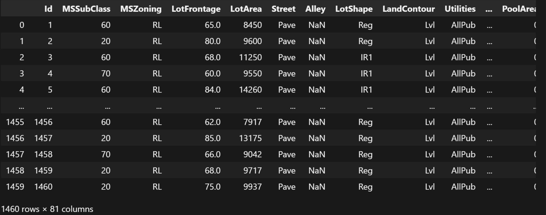
我们首先, 导入训练数据集:
import pandas as pd

data = pd.read_csv(
    r'./datas/house-prices-advanced-regression-techniques/train.csv')
data
这个训练数据集, 就在自己解压的目录下面, 路径根据自己解压的实际路径来。
结果:
接下来我们输出这么多变量之间的相关性(只展示数值类型的变量之间的相关性):
data_corr = data.corr(numeric_only=True)
data_corr
结果:
| Id | MSSubClass | LotFrontage | LotArea | OverallQual | OverallCond | YearBuilt | YearRemodAdd | MasVnrArea | BsmtFinSF1 | ... | WoodDeckSF | OpenPorchSF | EnclosedPorch | 3SsnPorch | ScreenPorch | PoolArea | MiscVal | MoSold | YrSold | SalePrice | |
|---|---|---|---|---|---|---|---|---|---|---|---|---|---|---|---|---|---|---|---|---|---|
| Id | 1.000000 | 0.011156 | -0.010601 | -0.033226 | -0.028365 | 0.012609 | -0.012713 | -0.021998 | -0.050298 | -0.005024 | ... | -0.029643 | -0.000477 | 0.002889 | -0.046635 | 0.001330 | 0.057044 | -0.006242 | 0.021172 | 0.000712 | -0.021917 |
| MSSubClass | 0.011156 | 1.000000 | -0.386347 | -0.139781 | 0.032628 | -0.059316 | 0.027850 | 0.040581 | 0.022936 | -0.069836 | ... | -0.012579 | -0.006100 | -0.012037 | -0.043825 | -0.026030 | 0.008283 | -0.007683 | -0.013585 | -0.021407 | -0.084284 |
| LotFrontage | -0.010601 | -0.386347 | 1.000000 | 0.426095 | 0.251646 | -0.059213 | 0.123349 | 0.088866 | 0.193458 | 0.233633 | ... | 0.088521 | 0.151972 | 0.010700 | 0.070029 | 0.041383 | 0.206167 | 0.003368 | 0.011200 | 0.007450 | 0.351799 |
| LotArea | -0.033226 | -0.139781 | 0.426095 | 1.000000 | 0.105806 | -0.005636 | 0.014228 | 0.013788 | 0.104160 | 0.214103 | ... | 0.171698 | 0.084774 | -0.018340 | 0.020423 | 0.043160 | 0.077672 | 0.038068 | 0.001205 | -0.014261 | 0.263843 |
| OverallQual | -0.028365 | 0.032628 | 0.251646 | 0.105806 | 1.000000 | -0.091932 | 0.572323 | 0.550684 | 0.411876 | 0.239666 | ... | 0.238923 | 0.308819 | -0.113937 | 0.030371 | 0.064886 | 0.065166 | -0.031406 | 0.070815 | -0.027347 | 0.790982 |
| OverallCond | 0.012609 | -0.059316 | -0.059213 | -0.005636 | -0.091932 | 1.000000 | -0.375983 | 0.073741 | -0.128101 | -0.046231 | ... | -0.003334 | -0.032589 | 0.070356 | 0.025504 | 0.054811 | -0.001985 | 0.068777 | -0.003511 | 0.043950 | -0.077856 |
| YearBuilt | -0.012713 | 0.027850 | 0.123349 | 0.014228 | 0.572323 | -0.375983 | 1.000000 | 0.592855 | 0.315707 | 0.249503 | ... | 0.224880 | 0.188686 | -0.387268 | 0.031355 | -0.050364 | 0.004950 | -0.034383 | 0.012398 | -0.013618 | 0.522897 |
| YearRemodAdd | -0.021998 | 0.040581 | 0.088866 | 0.013788 | 0.550684 | 0.073741 | 0.592855 | 1.000000 | 0.179618 | 0.128451 | ... | 0.205726 | 0.226298 | -0.193919 | 0.045286 | -0.038740 | 0.005829 | -0.010286 | 0.021490 | 0.035743 | 0.507101 |
| MasVnrArea | -0.050298 | 0.022936 | 0.193458 | 0.104160 | 0.411876 | -0.128101 | 0.315707 | 0.179618 | 1.000000 | 0.264736 | ... | 0.159718 | 0.125703 | -0.110204 | 0.018796 | 0.061466 | 0.011723 | -0.029815 | -0.005965 | -0.008201 | 0.477493 |
| BsmtFinSF1 | -0.005024 | -0.069836 | 0.233633 | 0.214103 | 0.239666 | -0.046231 | 0.249503 | 0.128451 | 0.264736 | 1.000000 | ... | 0.204306 | 0.111761 | -0.102303 | 0.026451 | 0.062021 | 0.140491 | 0.003571 | -0.015727 | 0.014359 | 0.386420 |
| BsmtFinSF2 | -0.005968 | -0.065649 | 0.049900 | 0.111170 | -0.059119 | 0.040229 | -0.049107 | -0.067759 | -0.072319 | -0.050117 | ... | 0.067898 | 0.003093 | 0.036543 | -0.029993 | 0.088871 | 0.041709 | 0.004940 | -0.015211 | 0.031706 | -0.011378 |
| BsmtUnfSF | -0.007940 | -0.140759 | 0.132644 | -0.002618 | 0.308159 | -0.136841 | 0.149040 | 0.181133 | 0.114442 | -0.495251 | ... | -0.005316 | 0.129005 | -0.002538 | 0.020764 | -0.012579 | -0.035092 | -0.023837 | 0.034888 | -0.041258 | 0.214479 |
| TotalBsmtSF | -0.015415 | -0.238518 | 0.392075 | 0.260833 | 0.537808 | -0.171098 | 0.391452 | 0.291066 | 0.363936 | 0.522396 | ... | 0.232019 | 0.247264 | -0.095478 | 0.037384 | 0.084489 | 0.126053 | -0.018479 | 0.013196 | -0.014969 | 0.613581 |
| 1stFlrSF | 0.010496 | -0.251758 | 0.457181 | 0.299475 | 0.476224 | -0.144203 | 0.281986 | 0.240379 | 0.344501 | 0.445863 | ... | 0.235459 | 0.211671 | -0.065292 | 0.056104 | 0.088758 | 0.131525 | -0.021096 | 0.031372 | -0.013604 | 0.605852 |
| 2ndFlrSF | 0.005590 | 0.307886 | 0.080177 | 0.050986 | 0.295493 | 0.028942 | 0.010308 | 0.140024 | 0.174561 | -0.137079 | ... | 0.092165 | 0.208026 | 0.061989 | -0.024358 | 0.040606 | 0.081487 | 0.016197 | 0.035164 | -0.028700 | 0.319334 |
| LowQualFinSF | -0.044230 | 0.046474 | 0.038469 | 0.004779 | -0.030429 | 0.025494 | -0.183784 | -0.062419 | -0.069071 | -0.064503 | ... | -0.025444 | 0.018251 | 0.061081 | -0.004296 | 0.026799 | 0.062157 | -0.003793 | -0.022174 | -0.028921 | -0.025606 |
| GrLivArea | 0.008273 | 0.074853 | 0.402797 | 0.263116 | 0.593007 | -0.079686 | 0.199010 | 0.287389 | 0.390857 | 0.208171 | ... | 0.247433 | 0.330224 | 0.009113 | 0.020643 | 0.101510 | 0.170205 | -0.002416 | 0.050240 | -0.036526 | 0.708624 |
| BsmtFullBath | 0.002289 | 0.003491 | 0.100949 | 0.158155 | 0.111098 | -0.054942 | 0.187599 | 0.119470 | 0.085310 | 0.649212 | ... | 0.175315 | 0.067341 | -0.049911 | -0.000106 | 0.023148 | 0.067616 | -0.023047 | -0.025361 | 0.067049 | 0.227122 |
| BsmtHalfBath | -0.020155 | -0.002333 | -0.007234 | 0.048046 | -0.040150 | 0.117821 | -0.038162 | -0.012337 | 0.026673 | 0.067418 | ... | 0.040161 | -0.025324 | -0.008555 | 0.035114 | 0.032121 | 0.020025 | -0.007367 | 0.032873 | -0.046524 | -0.016844 |
| FullBath | 0.005587 | 0.131608 | 0.198769 | 0.126031 | 0.550600 | -0.194149 | 0.468271 | 0.439046 | 0.276833 | 0.058543 | ... | 0.187703 | 0.259977 | -0.115093 | 0.035353 | -0.008106 | 0.049604 | -0.014290 | 0.055872 | -0.019669 | 0.560664 |
| HalfBath | 0.006784 | 0.177354 | 0.053532 | 0.014259 | 0.273458 | -0.060769 | 0.242656 | 0.183331 | 0.201444 | 0.004262 | ... | 0.108080 | 0.199740 | -0.095317 | -0.004972 | 0.072426 | 0.022381 | 0.001290 | -0.009050 | -0.010269 | 0.284108 |
| BedroomAbvGr | 0.037719 | -0.023438 | 0.263170 | 0.119690 | 0.101676 | 0.012980 | -0.070651 | -0.040581 | 0.102821 | -0.107355 | ... | 0.046854 | 0.093810 | 0.041570 | -0.024478 | 0.044300 | 0.070703 | 0.007767 | 0.046544 | -0.036014 | 0.168213 |
| KitchenAbvGr | 0.002951 | 0.281721 | -0.006069 | -0.017784 | -0.183882 | -0.087001 | -0.174800 | -0.149598 | -0.037610 | -0.081007 | ... | -0.090130 | -0.070091 | 0.037312 | -0.024600 | -0.051613 | -0.014525 | 0.062341 | 0.026589 | 0.031687 | -0.135907 |
| TotRmsAbvGrd | 0.027239 | 0.040380 | 0.352096 | 0.190015 | 0.427452 | -0.057583 | 0.095589 | 0.191740 | 0.280682 | 0.044316 | ... | 0.165984 | 0.234192 | 0.004151 | -0.006683 | 0.059383 | 0.083757 | 0.024763 | 0.036907 | -0.034516 | 0.533723 |
| Fireplaces | -0.019772 | -0.045569 | 0.266639 | 0.271364 | 0.396765 | -0.023820 | 0.147716 | 0.112581 | 0.249070 | 0.260011 | ... | 0.200019 | 0.169405 | -0.024822 | 0.011257 | 0.184530 | 0.095074 | 0.001409 | 0.046357 | -0.024096 | 0.466929 |
| GarageYrBlt | 0.000072 | 0.085072 | 0.070250 | -0.024947 | 0.547766 | -0.324297 | 0.825667 | 0.642277 | 0.252691 | 0.153484 | ... | 0.224577 | 0.228425 | -0.297003 | 0.023544 | -0.075418 | -0.014501 | -0.032417 | 0.005337 | -0.001014 | 0.486362 |
| GarageCars | 0.016570 | -0.040110 | 0.285691 | 0.154871 | 0.600671 | -0.185758 | 0.537850 | 0.420622 | 0.364204 | 0.224054 | ... | 0.226342 | 0.213569 | -0.151434 | 0.035765 | 0.050494 | 0.020934 | -0.043080 | 0.040522 | -0.039117 | 0.640409 |
| GarageArea | 0.017634 | -0.098672 | 0.344997 | 0.180403 | 0.562022 | -0.151521 | 0.478954 | 0.371600 | 0.373066 | 0.296970 | ... | 0.224666 | 0.241435 | -0.121777 | 0.035087 | 0.051412 | 0.061047 | -0.027400 | 0.027974 | -0.027378 | 0.623431 |
| WoodDeckSF | -0.029643 | -0.012579 | 0.088521 | 0.171698 | 0.238923 | -0.003334 | 0.224880 | 0.205726 | 0.159718 | 0.204306 | ... | 1.000000 | 0.058661 | -0.125989 | -0.032771 | -0.074181 | 0.073378 | -0.009551 | 0.021011 | 0.022270 | 0.324413 |
| OpenPorchSF | -0.000477 | -0.006100 | 0.151972 | 0.084774 | 0.308819 | -0.032589 | 0.188686 | 0.226298 | 0.125703 | 0.111761 | ... | 0.058661 | 1.000000 | -0.093079 | -0.005842 | 0.074304 | 0.060762 | -0.018584 | 0.071255 | -0.057619 | 0.315856 |
| EnclosedPorch | 0.002889 | -0.012037 | 0.010700 | -0.018340 | -0.113937 | 0.070356 | -0.387268 | -0.193919 | -0.110204 | -0.102303 | ... | -0.125989 | -0.093079 | 1.000000 | -0.037305 | -0.082864 | 0.054203 | 0.018361 | -0.028887 | -0.009916 | -0.128578 |
| 3SsnPorch | -0.046635 | -0.043825 | 0.070029 | 0.020423 | 0.030371 | 0.025504 | 0.031355 | 0.045286 | 0.018796 | 0.026451 | ... | -0.032771 | -0.005842 | -0.037305 | 1.000000 | -0.031436 | -0.007992 | 0.000354 | 0.029474 | 0.018645 | 0.044584 |
| ScreenPorch | 0.001330 | -0.026030 | 0.041383 | 0.043160 | 0.064886 | 0.054811 | -0.050364 | -0.038740 | 0.061466 | 0.062021 | ... | -0.074181 | 0.074304 | -0.082864 | -0.031436 | 1.000000 | 0.051307 | 0.031946 | 0.023217 | 0.010694 | 0.111447 |
| PoolArea | 0.057044 | 0.008283 | 0.206167 | 0.077672 | 0.065166 | -0.001985 | 0.004950 | 0.005829 | 0.011723 | 0.140491 | ... | 0.073378 | 0.060762 | 0.054203 | -0.007992 | 0.051307 | 1.000000 | 0.029669 | -0.033737 | -0.059689 | 0.092404 |
| MiscVal | -0.006242 | -0.007683 | 0.003368 | 0.038068 | -0.031406 | 0.068777 | -0.034383 | -0.010286 | -0.029815 | 0.003571 | ... | -0.009551 | -0.018584 | 0.018361 | 0.000354 | 0.031946 | 0.029669 | 1.000000 | -0.006495 | 0.004906 | -0.021190 |
| MoSold | 0.021172 | -0.013585 | 0.011200 | 0.001205 | 0.070815 | -0.003511 | 0.012398 | 0.021490 | -0.005965 | -0.015727 | ... | 0.021011 | 0.071255 | -0.028887 | 0.029474 | 0.023217 | -0.033737 | -0.006495 | 1.000000 | -0.145721 | 0.046432 |
| YrSold | 0.000712 | -0.021407 | 0.007450 | -0.014261 | -0.027347 | 0.043950 | -0.013618 | 0.035743 | -0.008201 | 0.014359 | ... | 0.022270 | -0.057619 | -0.009916 | 0.018645 | 0.010694 | -0.059689 | 0.004906 | -0.145721 | 1.000000 | -0.028923 |
| SalePrice | -0.021917 | -0.084284 | 0.351799 | 0.263843 | 0.790982 | -0.077856 | 0.522897 | 0.507101 | 0.477493 | 0.386420 | ... | 0.324413 | 0.315856 | -0.128578 | 0.044584 | 0.111447 | 0.092404 | -0.021190 | 0.046432 | -0.028923 | 1.000000 |
38 rows × 38 columns
接下来我们需要获取到跟房价这个变量最相关的10个属性:
top_features = data_corr['SalePrice'].abs().sort_values(ascending=False)[
    1:11]  # 获取最相关的前10个属性,这里我们是进行学习,所有不去细化分析了 正儿八经做的话 数据分析 研读文档 我们的重点是学习模型构建和训练
feature_cols = top_features.index.tolist() # 将取到的10个属性转换为列表
feature_cols
结果:
['OverallQual',
 'GrLivArea',
 'GarageCars',
 'GarageArea',
 'TotalBsmtSF',
 '1stFlrSF',
 'FullBath',
 'TotRmsAbvGrd',
 'YearBuilt',
 'YearRemodAdd']
除了上面的10个属性, 我们再对房子的信息进行补充:
feature_cols += [  # 房屋属性补充
    'HouseStyle',
    'ExterQual',
    'KitchenQual',
    # 区位与环境
    'Neighborhood',
    'LotArea',
    'LotFrontage',
    # 设施配套
    'CentralAir',
    'Fireplaces'
]
feature_cols
结果:
['OverallQual',
 'GrLivArea',
 'GarageCars',
 'GarageArea',
 'TotalBsmtSF',
 '1stFlrSF',
 'FullBath',
 'TotRmsAbvGrd',
 'YearBuilt',
 'YearRemodAdd',
 'HouseStyle',
 'ExterQual',
 'KitchenQual',
 'Neighborhood',
 'LotArea',
 'LotFrontage',
 'CentralAir',
 'Fireplaces']
将房价作为标签:
label_cols = ['SalePrice'] # 标记
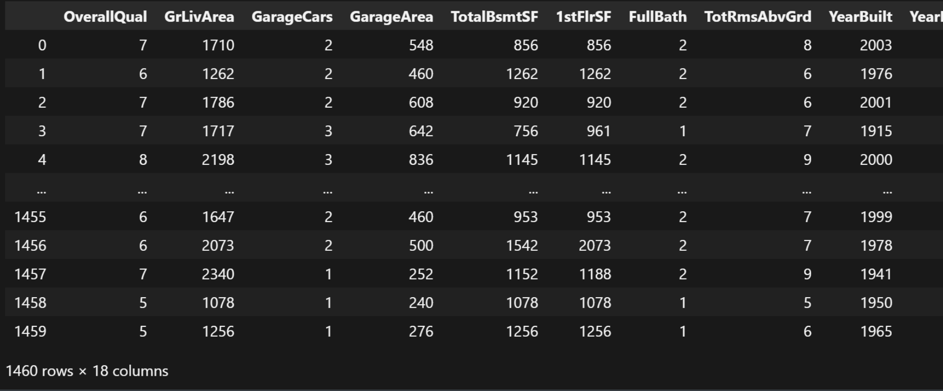
我们获取所有特征列的数据:
complete_data = data[feature_cols]
complete_data
结果:
我们接下来看一下数据总览, 检查有没有数据确实之类的问题:
complete_data.info()
结果:
<class 'pandas.core.frame.DataFrame'>
RangeIndex: 1460 entries, 0 to 1459
Data columns (total 18 columns):
 #   Column        Non-Null Count  Dtype
---  ------        --------------  -----
 0   OverallQual   1460 non-null   int64
 1   GrLivArea     1460 non-null   int64
 2   GarageCars    1460 non-null   int64
 3   GarageArea    1460 non-null   int64
 4   TotalBsmtSF   1460 non-null   int64
 5   1stFlrSF      1460 non-null   int64
 6   FullBath      1460 non-null   int64
 7   TotRmsAbvGrd  1460 non-null   int64
 8   YearBuilt     1460 non-null   int64
 9   YearRemodAdd  1460 non-null   int64
 10  HouseStyle    1460 non-null   object
 11  ExterQual     1460 non-null   object
 12  KitchenQual   1460 non-null   object
 13  Neighborhood  1460 non-null   object
 14  LotArea       1460 non-null   int64
 15  LotFrontage   1201 non-null   float64
 16  CentralAir    1460 non-null   object
 17  Fireplaces    1460 non-null   int64
dtypes: float64(1), int64(12), object(5)
memory usage: 205.4+ KB
果然, 我们发现的确有缺失值, LotFrontage只有1201条数据。
数据清洗和处理
我们对缺失值进行均值填充:
# 缺失值处理
complete_data = complete_data.copy()
complete_data['LotFrontage'] = complete_data['LotFrontage'].fillna(
    complete_data['LotFrontage'].mean())
complete_data.info()
结果:
<class 'pandas.core.frame.DataFrame'>
RangeIndex: 1460 entries, 0 to 1459
Data columns (total 18 columns):
 #   Column        Non-Null Count  Dtype
---  ------        --------------  -----
 0   OverallQual   1460 non-null   int64
 1   GrLivArea     1460 non-null   int64
 2   GarageCars    1460 non-null   int64
 3   GarageArea    1460 non-null   int64
 4   TotalBsmtSF   1460 non-null   int64
 5   1stFlrSF      1460 non-null   int64
 6   FullBath      1460 non-null   int64
 7   TotRmsAbvGrd  1460 non-null   int64
 8   YearBuilt     1460 non-null   int64
 9   YearRemodAdd  1460 non-null   int64
 10  HouseStyle    1460 non-null   object
 11  ExterQual     1460 non-null   object
 12  KitchenQual   1460 non-null   object
 13  Neighborhood  1460 non-null   object
 14  LotArea       1460 non-null   int64
 15  LotFrontage   1460 non-null   float64
 16  CentralAir    1460 non-null   object
 17  Fireplaces    1460 non-null   int64
dtypes: float64(1), int64(12), object(5)
memory usage: 205.4+ KB
缺失值填充好了之后, 我们需要记录关于特征列当中的数值类型的所有列:
# 记录数值类型的列
numeric_cols = complete_data.select_dtypes(include=['number']).columns
numeric_cols
结果:
Index(['OverallQual', 'GrLivArea', 'GarageCars', 'GarageArea', 'TotalBsmtSF',
       '1stFlrSF', 'FullBath', 'TotRmsAbvGrd', 'YearBuilt', 'YearRemodAdd',
       'LotArea', 'LotFrontage', 'Fireplaces'],
      dtype='object')
接下来, 我们需要进行独热编码的操作:
这里面的独热编码可以参考data_description.txt文件里面的说明。
# 对object进行独热编码
categorical_classes = {
    'HouseStyle': [
        '1Story', '1.5Fin', '1.5Unf', '2Story', '2.5Fin', '2.5Unf', 'SFoyer',
        'SLvl'
    ],
    'ExterQual': ['Ex', 'Gd', 'TA', 'Fa', 'Po'],
    'KitchenQual': ['Ex', 'Gd', 'TA', 'Fa', 'Po'],
    'Neighborhood': [
        'Blmngtn', 'Blueste', 'BrDale', 'BrkSide', 'ClearCr', 'CollgCr',
        'Crawfor', 'Edwards', 'Gilbert', 'IDOTRR', 'MeadowV', 'Mitchel',
        'Names', 'NoRidge', 'NPkVill', 'NridgHt', 'NWAmes', 'NAmes', 'OldTown',
        'SWISU', 'Sawyer', 'SawyerW', 'Somerst', 'StoneBr', 'Timber', 'Veenker'
    ],
    'CentralAir': ['N', 'Y']
}


def manual_one_hot_encode(df, categorical_features):
    encoded_rows = []  # 所有编码后的样本
    for _, row in df.iterrows():  # 获取每个样本的数据
        encoded_row = []  # 编码后的样本数据[]
        for feature in categorical_features:  # 要独热编码的每个特征
            value = row[feature]  # 选择要独热编码的特征值
            classes = categorical_classes[feature]  # 特征的所有可能值
            if value not in classes:  # 检查特征值是否在特征的所有可能值中
                print(row)
                raise ValueError(f'Value {value} not in classes {classes}')
            # 生成独热向量
            one_hot = [1 if value == class_ else 0 for class_ in classes]
            encoded_row.extend(one_hot)

        # 处理数值特征
        numerical_features = [
            col for col in df.columns if col not in categorical_features
        ]
        encoded_row.extend(row[numerical_features].values)
        encoded_rows.append(encoded_row)

    # 构建特征名
    feature_names = []
    for feature in categorical_features:
        feature_names.extend(
            [f'{feature}_{class_}' for class_ in categorical_classes[feature]])
    feature_names.extend(numerical_features)

    return pd.DataFrame(encoded_rows, columns=feature_names)


complete_data = manual_one_hot_encode(complete_data, categorical_classes)
complete_data
这里, 我们对所有的特征属性都进行了独热编码的处理。
独热编码的基本原理:
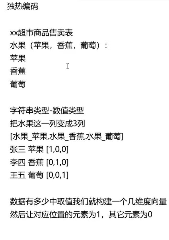
独热编码的缺点: 如果数据的取值范围非常大(可能性值)很多的时候, 会造成维度爆炸。
运行结果:
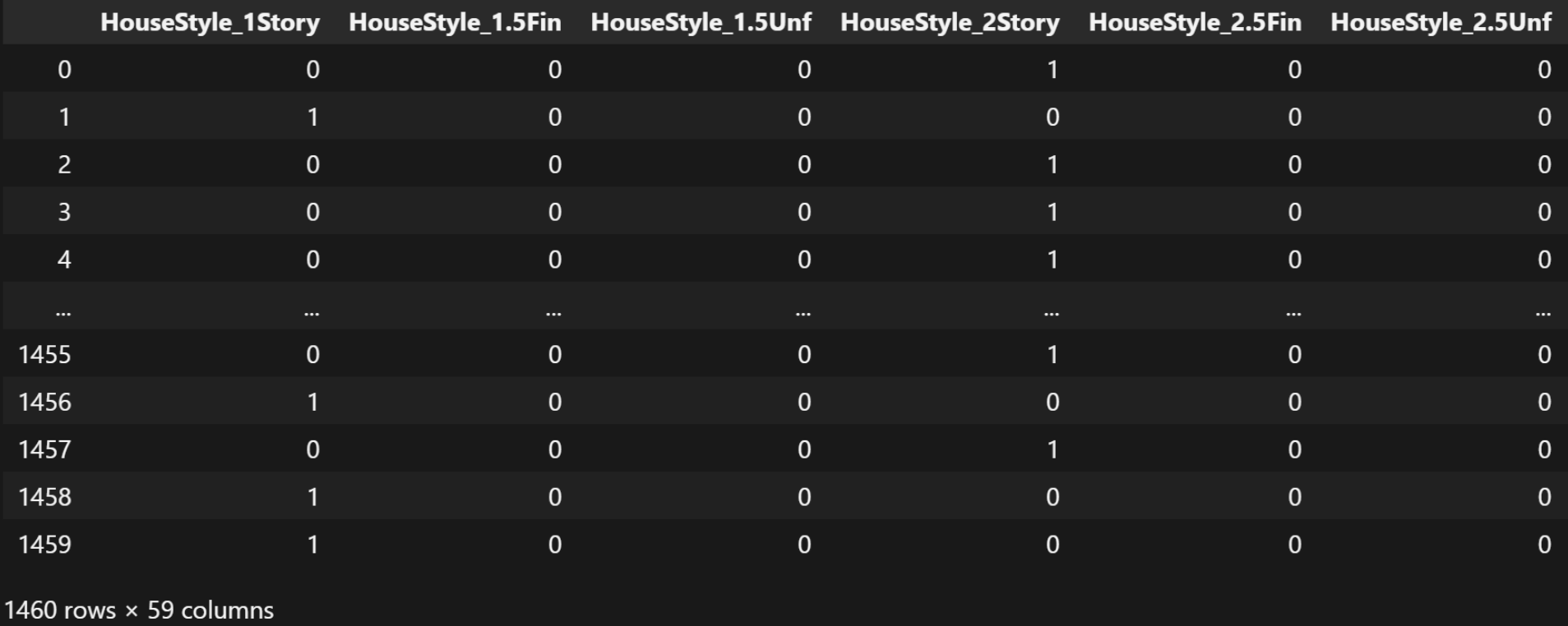
独热编码的结果只有0和1。
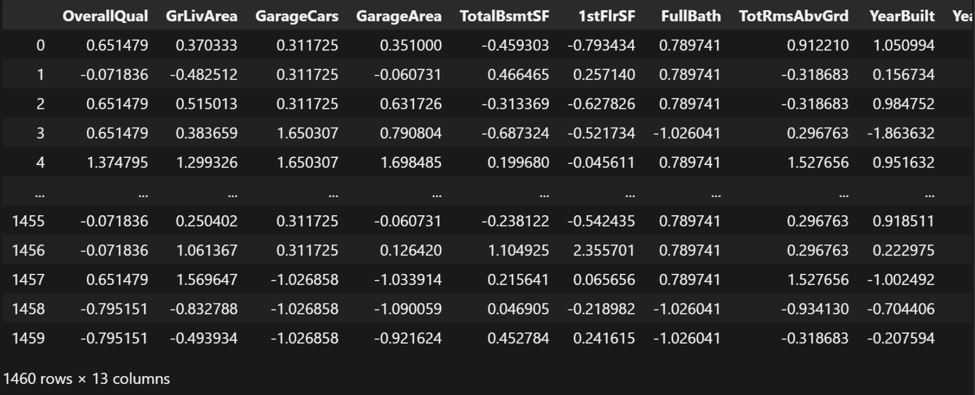
我们接下来需要给那些数值类型的那些列进行标准化:
from sklearn.preprocessing import StandardScaler

X_strandard = StandardScaler()

# 单独给原来的数值列进行标准化
X_strandard_data = pd.DataFrame(X_strandard.fit_transform(
    complete_data[numeric_cols]),
                                columns=numeric_cols)
X_strandard_data
结果:
接下来我们需要获取除了数值类型的其它所有的列名:
# 获取除去numeric_cols的其它列名
other_cols = complete_data.columns.difference(numeric_cols)
other_cols
结果:
Index(['CentralAir_N', 'CentralAir_Y', 'ExterQual_Ex', 'ExterQual_Fa',
       'ExterQual_Gd', 'ExterQual_Po', 'ExterQual_TA', 'HouseStyle_1.5Fin',
       'HouseStyle_1.5Unf', 'HouseStyle_1Story', 'HouseStyle_2.5Fin',
       'HouseStyle_2.5Unf', 'HouseStyle_2Story', 'HouseStyle_SFoyer',
       'HouseStyle_SLvl', 'KitchenQual_Ex', 'KitchenQual_Fa', 'KitchenQual_Gd',
       'KitchenQual_Po', 'KitchenQual_TA', 'Neighborhood_Blmngtn',
       'Neighborhood_Blueste', 'Neighborhood_BrDale', 'Neighborhood_BrkSide',
       'Neighborhood_ClearCr', 'Neighborhood_CollgCr', 'Neighborhood_Crawfor',
       'Neighborhood_Edwards', 'Neighborhood_Gilbert', 'Neighborhood_IDOTRR',
       'Neighborhood_MeadowV', 'Neighborhood_Mitchel', 'Neighborhood_NAmes',
       'Neighborhood_NPkVill', 'Neighborhood_NWAmes', 'Neighborhood_Names',
       'Neighborhood_NoRidge', 'Neighborhood_NridgHt', 'Neighborhood_OldTown',
       'Neighborhood_SWISU', 'Neighborhood_Sawyer', 'Neighborhood_SawyerW',
       'Neighborhood_Somerst', 'Neighborhood_StoneBr', 'Neighborhood_Timber',
       'Neighborhood_Veenker'],
      dtype='object')
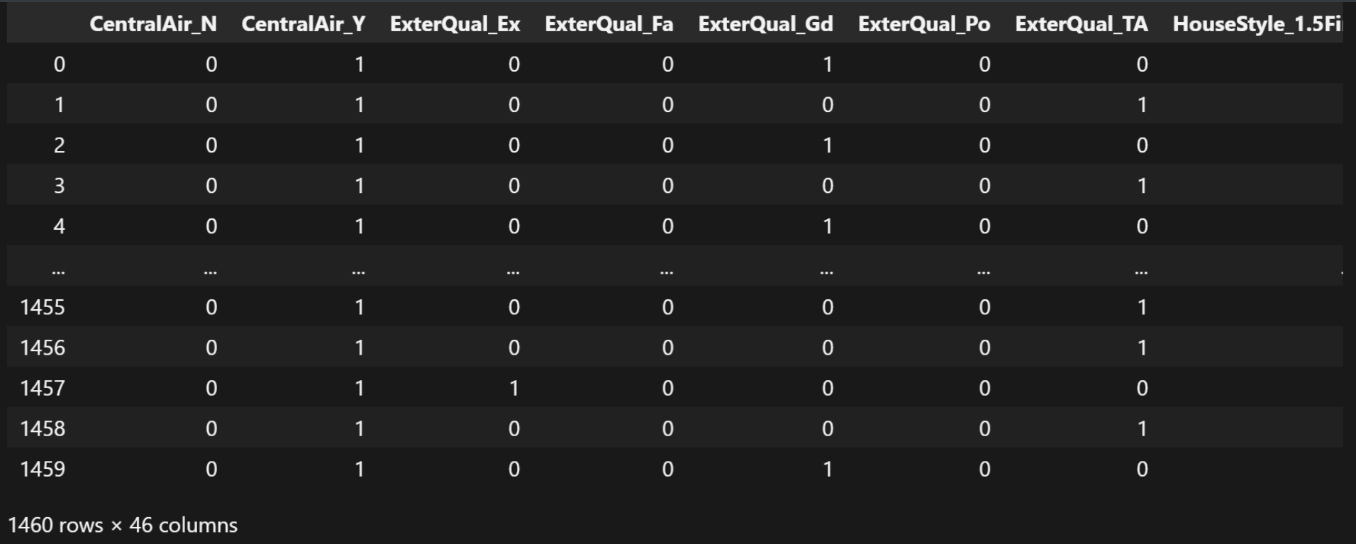
获取刚才获取到所有列的信息(就是出数值类型以外所有类的值):
# 获取complete_data中的other_cols列的数据
other_cols_data = complete_data[other_cols]
other_cols_data
结果:
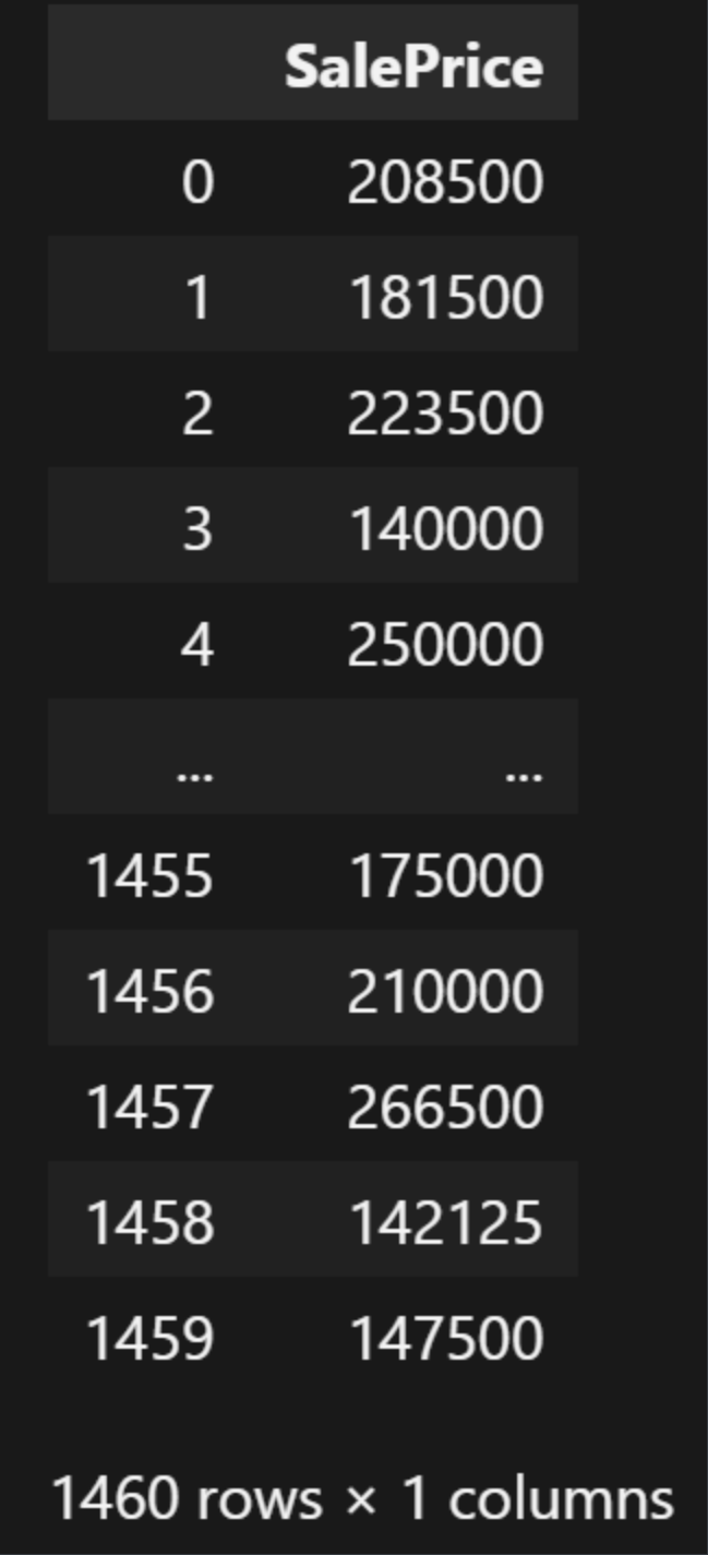
我们获取房价那一列数据:
# 标签列
Y_strandard_data = pd.DataFrame(data[label_cols], columns=label_cols)
Y_strandard_data
结果:
合并数据(这里合并后的数据是数值类型的特征标准化后的结果+非数值类数据进行独热编码后的结果+房价数据):
# 合并 标准化的数值列和独热编码列和标签列
merged_data = pd.concat([X_strandard_data, other_cols_data, Y_strandard_data],
                        axis=1)
merged_data
结果:
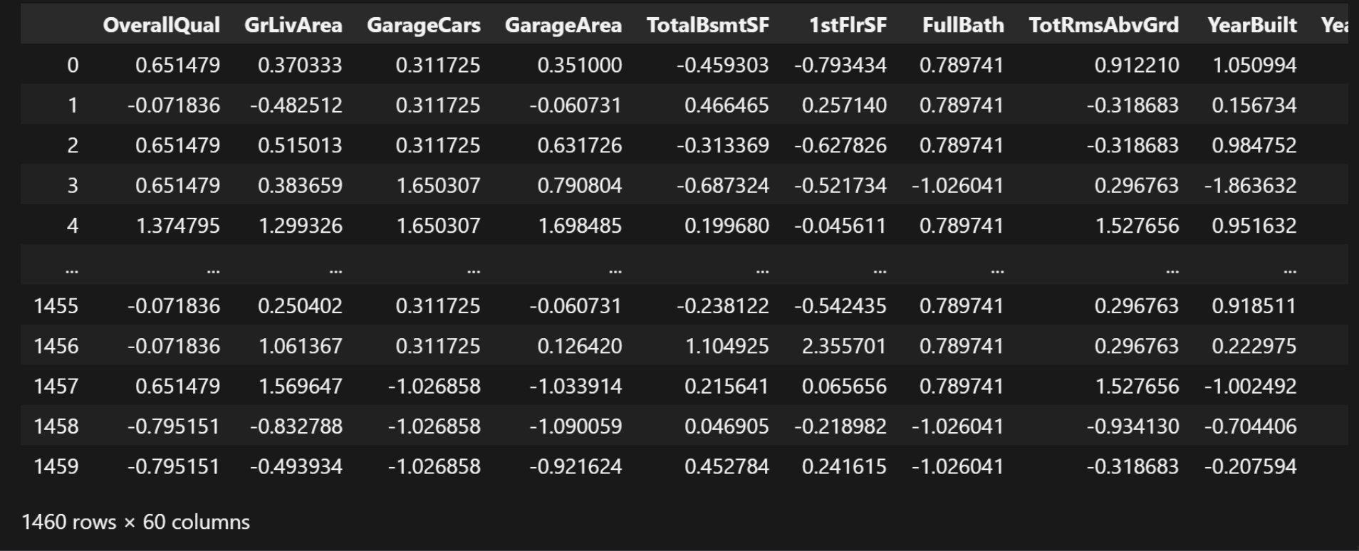
合并完数据之后有60列数据
最终我们把处理好的数据保存到csv文件里面去:
merged_data.to_csv('train.csv', index=False)
模型训练
首先, 我们还是一样, 得先"固定随机性", 目的是让实验可复现:
import numpy as np
import torch


def seed_everything(seed=42):
    np.random.seed(seed)
    torch.manual_seed(seed)
    torch.cuda.manual_seed(seed)
    torch.cuda.manual_seed_all(seed)
    torch.backends.cudnn.deterministic = True
    torch.backends.cudnn.benchmark = False


seed_everything()
随后我们导入我们刚在已经处理好的数据:
import pandas as pd

train_data = pd.read_csv('train.csv')
train_data
划分数据与标签:
# 特征和标签
X_strandard_data = train_data.drop('SalePrice',
                                   axis=1)  # 对dataframe做删除-dataframe
Y_strandard_data = train_data['SalePrice']  # 去dataframe的一列-series
X_strandard_data
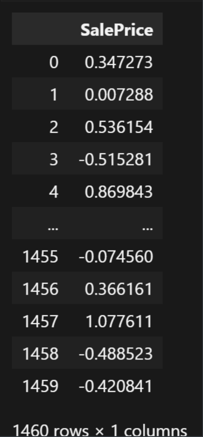
我们对房价的数据进行标准化:
from sklearn.preprocessing import StandardScaler

Y_trandard = StandardScaler()
Y_standard_data = pd.DataFrame(Y_trandard.fit_transform(
    Y_strandard_data.to_frame()),
                               columns=['SalePrice'])
Y_standard_data
划分训练集和验证集数据:
from sklearn.model_selection import train_test_split

X_train, X_test, y_train, y_test = train_test_split(X_strandard_data,
                                                    Y_standard_data,
                                                    test_size=0.3)
X_train
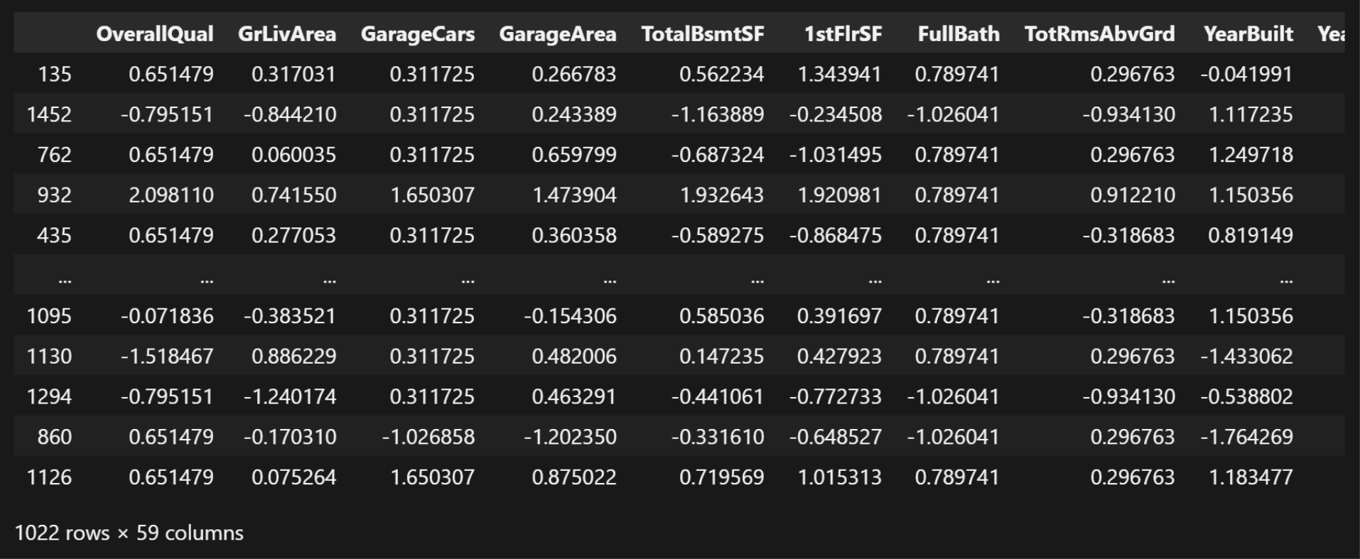
这里面我们可以发现, 训练集有59列,测试机只有1列(房价)。这里面的test_size=0.3指的是在这里面的所有数据当中取30%当作验证机数据。
利用GPU去跑模型:
import torch

device = torch.device('cuda' if torch.cuda.is_available() else 'cpu')
device
结果:
device(type='cuda')
将划分好的训练集和测试集数据全部都用GPU去训练:
X_train_tensor = torch.tensor(X_train.values, dtype=torch.float32).to(device)
y_train_tensor = torch.tensor(y_train.values, dtype=torch.float32).to(device)
X_test_tensor = torch.tensor(X_test.values, dtype=torch.float32).to(device)
y_test_tensor = torch.tensor(y_test.values, dtype=torch.float32).to(device)
X_train_tensor.shape
结果:
torch.Size([1022, 59])
使用加载器批量加载训练集数据, 以[特征-标签]为格式:
from torch.utils.data import TensorDataset, DataLoader

train_dataset = TensorDataset(X_train_tensor, y_train_tensor)  # [特征-标签]
train_loader = DataLoader(
    train_dataset, batch_size=64,
    shuffle=True)  # DataLoader 数据加载器 批量划分 batch_size=64 64个样本为一组
len(train_loader)
结果:
16
我们可以提取一个示例来检查验证:
# 提取一个示例来检查验证
examples = enumerate(train_loader)  # [(0,[特征,标签]),()]
batch_idx, (example_data, example_targets) = next(examples)
batch_idx, example_data.shape, example_targets.shape
结果:
(0, torch.Size([64, 59]), torch.Size([64, 1]))
训练集和测试集的第一行数据:
example_data[0], example_targets[0]
结果:
(tensor([ 0.6515, -0.1665,  0.3117,  0.3791,  0.8199,  0.6867,  0.7897, -0.3187,
          1.2166,  1.1209,  0.1761,  0.9516, -0.9512,  0.0000,  1.0000,  0.0000,
          0.0000,  1.0000,  0.0000,  0.0000,  0.0000,  0.0000,  1.0000,  0.0000,
          0.0000,  0.0000,  0.0000,  0.0000,  1.0000,  0.0000,  0.0000,  0.0000,
          0.0000,  0.0000,  0.0000,  0.0000,  0.0000,  0.0000,  0.0000,  0.0000,
          0.0000,  0.0000,  0.0000,  0.0000,  0.0000,  0.0000,  0.0000,  0.0000,
          0.0000,  0.0000,  0.0000,  0.0000,  0.0000,  0.0000,  0.0000,  1.0000,
          0.0000,  0.0000,  0.0000], device='cuda:0'),
 tensor([0.5888], device='cuda:0'))
构建模型:
from torch import nn


class HousePriceModel(nn.Module):

    def __init__(self, input_size) -> None:
        super().__init__()
        self.linear1 = nn.Linear(input_size, 128)  # 59->128
        self.linear2 = nn.Linear(128, 256)
        self.linear3 = nn.Linear(256, 128)
        self.linear4 = nn.Linear(128, 64)
        self.output = nn.Linear(64, 1)  # 64->1
        self.relu = nn.ReLU()
        self.droupt = nn.Dropout(0.2)  # p=0.2 丢弃20%的神经元信息

    def forward(self, x):
        x = self.relu(self.linear1(x))
        x = self.droupt(x)

        x = self.relu(self.linear2(x))
        x = self.droupt(x)

        x = self.relu(self.linear3(x))
        x = self.droupt(x)

        x = self.relu(self.linear4(x))
        return self.output(x)  # 注意,输出层不需要激活函数


model = HousePriceModel(X_train_tensor.shape[-1])
model.to(device)
这里面我们使用ReLU激活函数, 还有利用多线性层来构建模型, 包括在后面也用上了Dropout, 丢弃神经元, 也就是说我们可以让模型抛弃掉一部分内容去学习, 不然的话模型很容易过拟合。(简单的来说就是不要让模型学的太死板, 不需要学习到的那些细节就不用让模型去学习)
构建出来模型的结果:
HousePriceModel(
  (linear1): Linear(in_features=59, out_features=128, bias=True)
  (linear2): Linear(in_features=128, out_features=256, bias=True)
  (linear3): Linear(in_features=256, out_features=128, bias=True)
  (linear4): Linear(in_features=128, out_features=64, bias=True)
  (output): Linear(in_features=64, out_features=1, bias=True)
  (relu): ReLU()
  (droupt): Dropout(p=0.2, inplace=False)
)
我们可以查看下这个模型的总参数有多少:
total_params = sum(p.numel() for p in model.parameters() if p.requires_grad)
print('模型总参数:', total_params)
结果:
模型总参数: 81921
构建损失函数
我们还是构建一个MSE均方误差的函数
criterion = nn.MSELoss() # 回归-MSE
构建一个优化器
from torch import optim

optimizer = optim.SGD(model.parameters(), lr=1e-3, weight_decay=1e-5)  # L2正则化
这里面的1e-3代表1乘以10的(-3)次方, 这里面用的是科学计数法, 1e-5也是同理。
lr是学习率, weight_decay就是权重衰减。
训练模型
num_epochs = 2000

train_losses = []
test_losses = []

patience = 100  # 早停耐心值,如果验证的损失在100次训练中都没有提升,则停止训练
best_val_loss = float('inf')  # 初始化无穷大

best_model_path = r'./models/best_housing_model01.pth'
我们设置让模型训练2000次, 当模型训练的过程中, 发现有连续训练100次且一直没有提升的情况, 那就需要立即停止模型训练, 否则会导致模型的过拟合。
训练代码:
for epoch in range(num_epochs):
    model.train()
    epoch_loss = 0  # 每个epoch的损失 每个批次的总损失
    for batch_X, batch_y in train_loader:

        # 对每个批次进行训练
        y_pred = model(batch_X)

        loss = criterion(y_pred, batch_y)
        epoch_loss += loss.item()

        optimizer.zero_grad()
        loss.backward()
        optimizer.step()
    avg_train_loss = epoch_loss / len(train_loader)
    train_losses.append(avg_train_loss)

    model.eval()
    with torch.no_grad():
        y_pred_all = model(X_test_tensor)
        val_loss = criterion(y_pred_all, y_test_tensor)
        test_losses.append(val_loss.item())

    if (epoch + 1) % 10 == 0:
        print(
            f"Epoch {epoch+1}/{num_epochs}, Train Loss: {avg_train_loss:.4f}, Test Loss: {val_loss:.4f}"
        )

    if val_loss < best_val_loss:
        best_val_loss = val_loss
        counter = 0  # 重置计数器
        # 保存模型参数
        torch.save(model.state_dict(), best_model_path)
        print(
            f"Best model saved at Epoch {epoch+1}, Train Loss: {avg_train_loss:.4f}, Test Loss: {val_loss:.4f}"
        )
    else:
        # 本次训练没有提升
        counter += 1  # 累计没有提升的次数
        if counter >= patience:
            print(f"Early stopping at Epoch {epoch+1}")
            break
这里面有训练集和验证机的损失记录, 并且还把每一次训练的最佳结果, 都保存到了文件里面。
结果:
Best model saved at Epoch 1, Train Loss: 0.9627, Test Loss: 1.1129
Best model saved at Epoch 2, Train Loss: 0.9615, Test Loss: 1.1121
Best model saved at Epoch 3, Train Loss: 0.9609, Test Loss: 1.1113
Best model saved at Epoch 4, Train Loss: 0.9595, Test Loss: 1.1104
Best model saved at Epoch 5, Train Loss: 0.9590, Test Loss: 1.1096
Best model saved at Epoch 6, Train Loss: 0.9583, Test Loss: 1.1088
Best model saved at Epoch 7, Train Loss: 0.9567, Test Loss: 1.1080
Best model saved at Epoch 8, Train Loss: 0.9556, Test Loss: 1.1072
Best model saved at Epoch 9, Train Loss: 0.9561, Test Loss: 1.1065
Epoch 10/2000, Train Loss: 0.9552, Test Loss: 1.1057
Best model saved at Epoch 10, Train Loss: 0.9552, Test Loss: 1.1057
Best model saved at Epoch 11, Train Loss: 0.9567, Test Loss: 1.1049
Best model saved at Epoch 12, Train Loss: 0.9553, Test Loss: 1.1041
Best model saved at Epoch 13, Train Loss: 0.9522, Test Loss: 1.1034
Best model saved at Epoch 14, Train Loss: 0.9521, Test Loss: 1.1026
Best model saved at Epoch 15, Train Loss: 0.9520, Test Loss: 1.1018
Best model saved at Epoch 16, Train Loss: 0.9524, Test Loss: 1.1011
Best model saved at Epoch 17, Train Loss: 0.9506, Test Loss: 1.1003
Best model saved at Epoch 18, Train Loss: 0.9493, Test Loss: 1.0995
Best model saved at Epoch 19, Train Loss: 0.9506, Test Loss: 1.0988
Epoch 20/2000, Train Loss: 0.9479, Test Loss: 1.0980
Best model saved at Epoch 20, Train Loss: 0.9479, Test Loss: 1.0980
Best model saved at Epoch 21, Train Loss: 0.9478, Test Loss: 1.0972
Best model saved at Epoch 22, Train Loss: 0.9472, Test Loss: 1.0964
Best model saved at Epoch 23, Train Loss: 0.9472, Test Loss: 1.0956
...
Epoch 1970/2000, Train Loss: 0.1088, Test Loss: 0.1025
Epoch 1980/2000, Train Loss: 0.1096, Test Loss: 0.1034
Epoch 1990/2000, Train Loss: 0.1277, Test Loss: 0.1026
Epoch 2000/2000, Train Loss: 0.1217, Test Loss: 0.1022
Output is truncated. View as a scrollable element or open in a text editor. Adjust cell output settings...
接下来我们需要画图, 查看该模型训练的结果(训练损失值和验证损失值):
import matplotlib.pyplot as plt
import seaborn as sns

sns.set_theme()
plt.figure(figsize=(10, 6))
plt.plot(train_losses, label='Train Loss')  # x轴是训练的轮次,y轴是对应轮次的对应损失
plt.plot(test_losses, label='Val Loss')
plt.xlabel('Epoch')
plt.ylabel('Loss')
plt.legend()
plt.show()
结果:
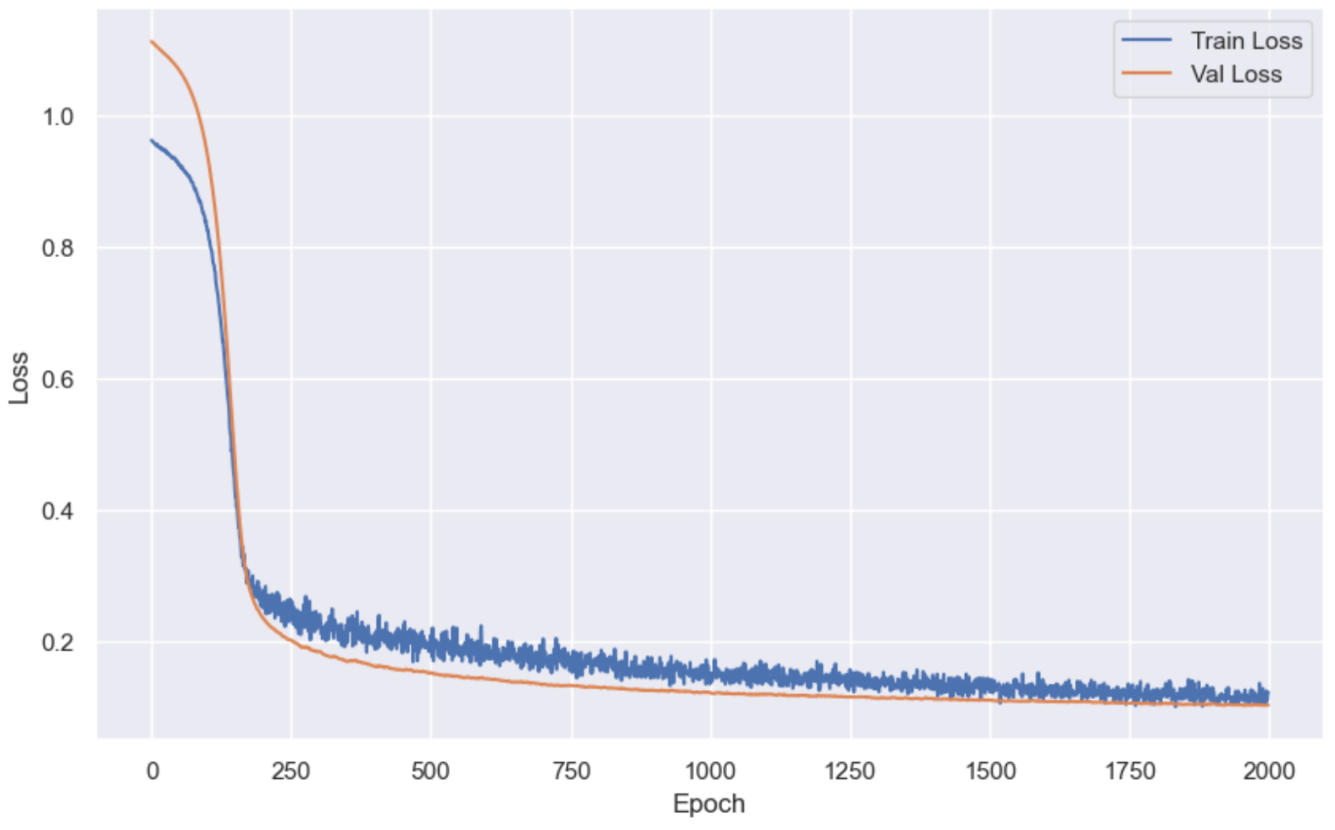
到这里我们的模型就训练完毕了, 接下来我们就可以开始应用模型了。
我们可以加载刚才我们训练好的模型:
model.load_state_dict(
    torch.load(best_model_path)
)  # Best model saved at Epoch 1766, Train Loss: 0.0578, Test Loss: 0.0933
model.eval()
with torch.no_grad():
    y_pred_all = model(X_test_tensor)

y_pred_all[:10], y_test_tensor[:10]
加载模型, 并且让模型去预测房价, 然后再和真实房价做对比。
结果:
(tensor([[-0.5304],
         [ 2.0108],
         [-0.7652],
         [-0.3480],
         [ 1.6332],
         [-1.3117],
         [ 0.7818],
         [-0.4620],
         [-1.3179],
         [-0.6735]], device='cuda:0'),
 tensor([[-0.3327],
         [ 1.8142],
         [-0.8301],
         [-0.2760],
         [ 1.6946],
         [-1.3275],
         [ 1.6443],
         [-0.4397],
         [-1.2141],
         [-0.5719]], device='cuda:0'))
由于标准化过后的数据, 不容易读懂, 所以我们需要进行反标准化处理。
Y_pred_inverse = Y_trandard.inverse_transform(y_pred_all.cpu().numpy())
Y_test_inverse = Y_trandard.inverse_transform(y_test_tensor.cpu().numpy())
Y_pred_inverse[:10], Y_test_inverse[:10]
结果:
(array([[138798.42 ],
        [340608.25 ],
        [120148.86 ],
        [153285.45 ],
        [310623.2  ],
        [ 76752.805],
        [243004.47 ],
        [144227.47 ],
        [ 76255.9  ],
        [127434.375]], dtype=float32),
 array([[154500.],
        [325000.],
        [115000.],
        [159000.],
        [315500.],
        [ 75500.],
        [311500.],
        [146000.],
        [ 84500.],
        [135500.]], dtype=float32))
最后我们再画张图, 来对比一下模型预测的结果和房价真实的结果:
plt.figure(figsize=(10, 6))
plt.scatter(Y_test_inverse, Y_pred_inverse, alpha=0.5)
plt.plot([min(Y_test_inverse), max(Y_test_inverse)],
         [min(Y_test_inverse), max(Y_test_inverse)],
         color='red',
         linewidth=2)
plt.xlabel('Actual SalePrice')
plt.ylabel('Predicted SalePrice')
plt.title('Actual vs Predicted SalePrice')
plt.grid(True)
plt.show()
结果:
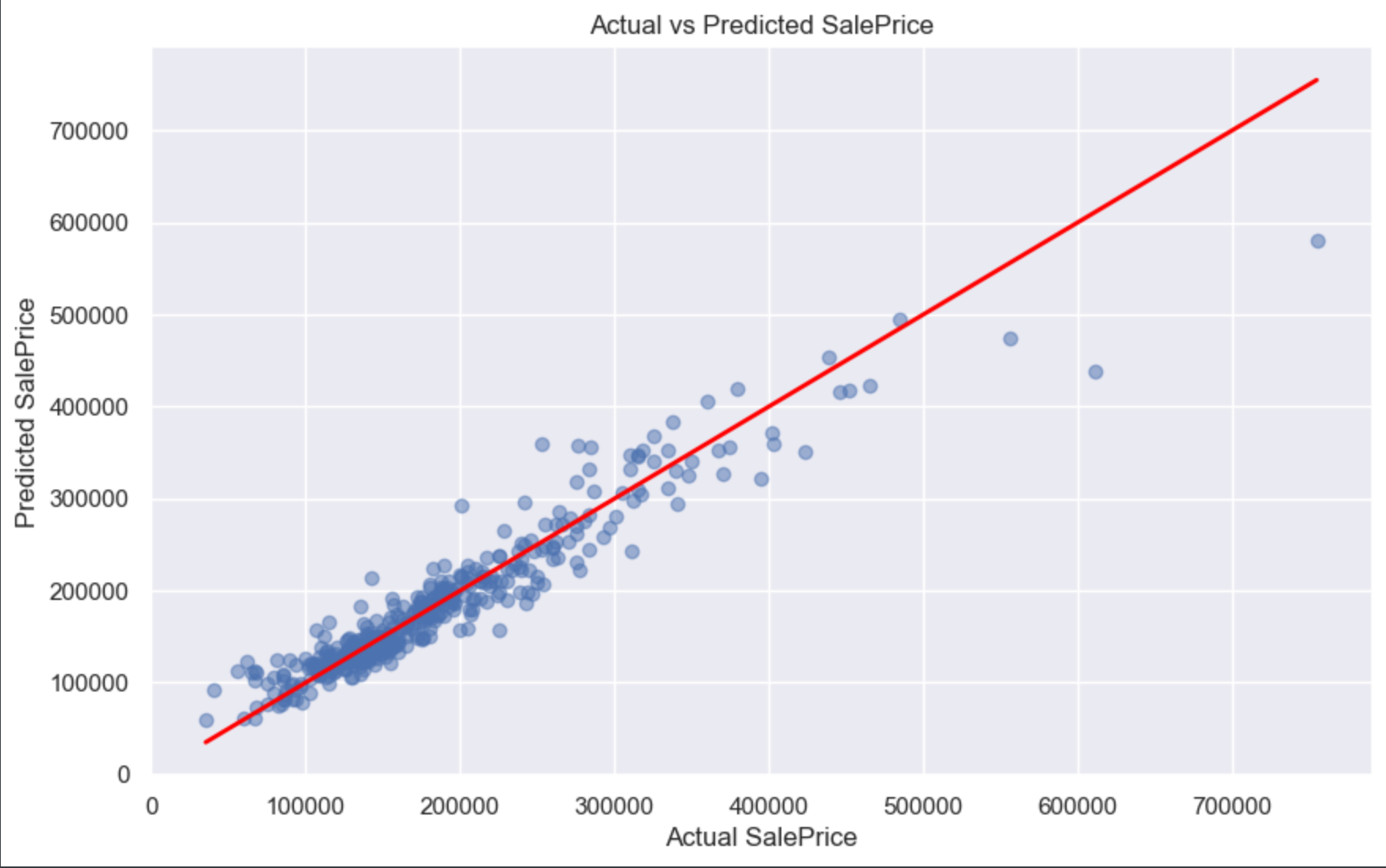
我们可以很清晰的看到, 红色线就是模型预测出来的结果, 而那些蓝色的透明点就是房价真实值。
这里我需要交给大家一个任务: 做实验 - 调整现有模型的超参数和模型结构,看模型的损失还能不能继续降低(你修改特征也是没问题)。如果大家的实验有做出成果了, 可以截图或以文字信息(代码也没问题)发在评论区。
好了, 关于这篇模型提升的内容就到此结束了。那关于线性回归的内容, 也就到此结束了, 接下来的文章, 会讲解关于逻辑回归的内容。
以上就是模型提升的所有内容了, 如果有哪里不懂的地方,可以把问题打在评论区, 欢迎大家在评论区交流!!!
如果我有写错的地方, 望大家指正, 也可以联系我, 让我们一起努力, 继续不断的进步.
学习是个漫长的过程, 需要我们不断的去学习并掌握消化知识点, 有不懂或概念模糊不理解的情况下,一定要赶紧的解决问题, 否则问题只会越来越多, 漏洞也就越老越大.
人生路漫漫, 白鹭常相伴!!!

有“AI”的1024 = 2048,欢迎大家加入2048 AI社区
更多推荐


 15
15 0
0- 0


 已为社区贡献2条内容

所有评论(0)