从 Ascend C Kernel 到 AI 框架调用 - 算子集成与编译部署全流程深度解析
本文基于CANN量化Matmul开发样例,系统解析从Ascend C Kernel编写到AI框架调用的完整技术链路。我将深入探讨ops-nn算子库架构、NPU硬件特性如何影响算子设计、量化矩阵乘的Tiling策略与Kernel实现,以及算子如何通过ATC编译、集成到PyTorch/TensorFlow等框架。通过实际开发案例展示从硬件特性到软件生态的垂直整合,提供可落地的算子开发部署方法论。硬件感
目录
🎯 摘要
本文基于CANN量化Matmul开发样例,系统解析从Ascend C Kernel编写到AI框架调用的完整技术链路。我将深入探讨ops-nn算子库架构、NPU硬件特性如何影响算子设计、量化矩阵乘的Tiling策略与Kernel实现,以及算子如何通过ATC编译、集成到PyTorch/TensorFlow等框架。通过实际开发案例展示从硬件特性到软件生态的垂直整合,提供可落地的算子开发部署方法论。
1. CANN算子生态的垂直整合哲学
1.1 🔄 ops-nn算子库:CANN的神经网络计算核心
在我13年的芯片系统开发经历中,真正理解一个芯片生态的成功关键,不在于硬件峰值算力,而在于算子库的完备性和易用性。CANN的ops-nn仓正是这一理念的集中体现。
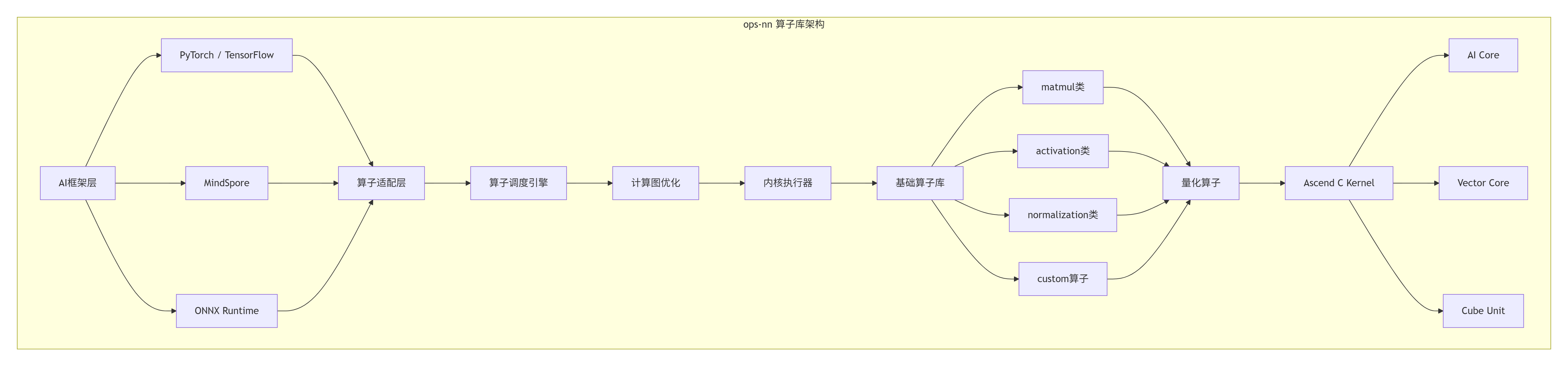
ops-nn设计洞察:
-
模块化分层:上层框架无关,下层硬件优化
-
统一接口抽象:屏蔽硬件差异,提供一致API
-
性能可移植:同一算子在不同昇腾芯片上自动优化
1.2 📊 矩阵乘:NPU的"底层计算引擎"
在Transformer一统AI江湖的今天,矩阵乘已不再是简单的线性代数运算,而是整个AI计算体系的基石。CANN中的矩阵乘实现,体现了软硬协同的深度优化。
# 矩阵乘在AI模型中的关键作用分析
class MatmulImportanceAnalyzer:
    def analyze_model_composition(self, model_name: str):
        """分析模型中矩阵乘的占比"""
        models = {
            "BERT-Large": {
                "total_ops": 3.3e9,  # 33亿次操作
                "matmul_ops": 2.4e9,  # 24亿次矩阵乘
                "percentage": 72.7,   # 占比72.7%
                "key_layers": ["Attention", "FFN"]
            },
            "GPT-3 175B": {
                "total_ops": 1.75e12,  # 1.75万亿次操作
                "matmul_ops": 1.4e12,  # 1.4万亿次矩阵乘
                "percentage": 80.0,    # 占比80%
                "key_layers": ["QKV_Proj", "Attention", "FFN"]
            },
            "ResNet-50": {
                "total_ops": 3.9e9,   # 39亿次操作
                "matmul_ops": 0.8e9,  # 8亿次矩阵乘
                "percentage": 20.5,   # 占比20.5%
                "key_layers": ["FC", "1x1 Conv"]
            }
        }

        return models.get(model_name, {})

# 量化矩阵乘的性能优势
def quant_matmul_benefits():
    """量化矩阵乘的性能收益分析"""
    benefits = {
        "性能提升": {
            "INT8 vs FP32": "3-4倍理论加速",
            "INT8 vs FP16": "1.5-2倍加速",
            "实际模型端到端": "1.8-2.5倍加速"
        },
        "内存节省": {
            "权重内存": "减少75%",
            "激活值内存": "减少50%",
            "缓存需求": "减少60%"
        },
        "功耗降低": {
            "计算功耗": "降低60-70%",
            "内存访问功耗": "降低50%",
            "总系统功耗": "降低40-50%"
        }
    }
    return benefits
2. NPU硬件架构:算子设计的物理基础
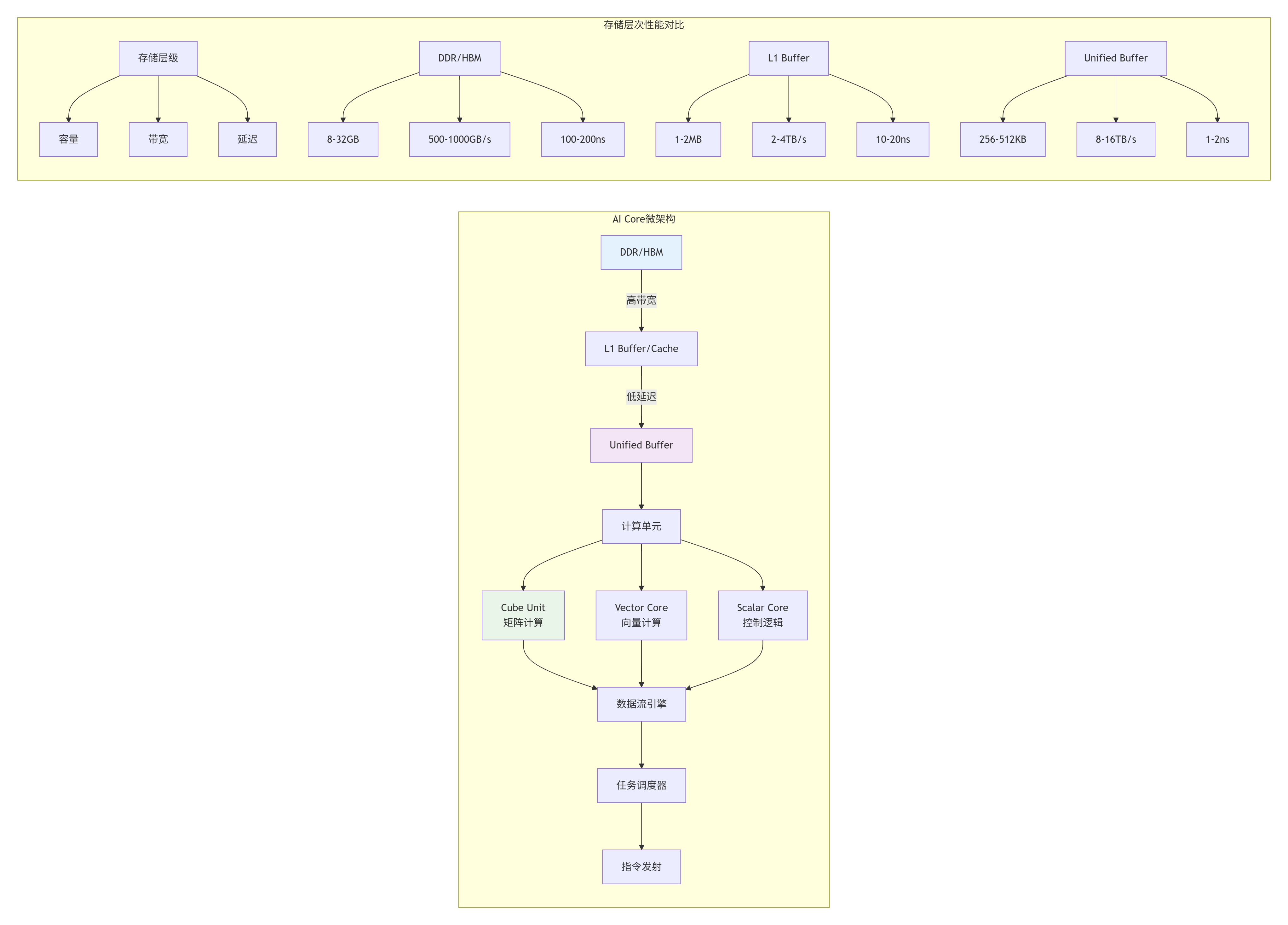
2.1 🔧 AI Core与存储单元的协同设计
真正高效的算子设计,必须从硬件架构出发。昇腾NPU的AI Core设计体现了计算密度优先、内存层次优化、数据流驱动三大原则。
2.2 ⚡ 量化矩阵乘的硬件映射策略
// QuantBatchMatmulV3的硬件感知设计
// 文件:quant_matmul_hardware_aware.c
// Ascend C 版本: 1.3+

#include <ascendc.h>

// 基于硬件特性的配置参数
struct HardwareAwareConfig {
    // AI Core配置
    int cube_unit_size;      // Cube单元大小 (16x16)
    int vector_unit_width;   // 向量单元宽度 (256-bit)
    int unified_buffer_size; // Unified Buffer大小 (256KB)
    int register_count;      // 寄存器数量 (256)

    // 内存层级配置
    int l1_cache_size;       // L1缓存大小 (1MB)
    int l1_cache_line;       // 缓存行大小 (128B)
    int memory_alignment;    // 内存对齐要求 (128B)

    // 性能优化参数
    int optimal_tile_m;      // 最优M方向分块
    int optimal_tile_n;      // 最优N方向分块
    int optimal_tile_k;      // 最优K方向分块
    int double_buffer_size;  // 双缓冲大小
};

// 自动硬件探测与配置
__aicore__ HardwareAwareConfig detect_hardware_config() {
    HardwareAwareConfig config;

    // 探测硬件特性
    config.cube_unit_size = get_hardware_feature(HW_FEATURE_CUBE_SIZE);
    config.vector_unit_width = get_hardware_feature(HW_FEATURE_VECTOR_WIDTH);
    config.unified_buffer_size = get_hardware_feature(HW_FEATURE_UB_SIZE);
    config.register_count = get_hardware_feature(HW_FEATURE_REGISTER_COUNT);

    config.l1_cache_size = get_hardware_feature(HW_FEATURE_L1_SIZE);
    config.l1_cache_line = get_hardware_feature(HW_FEATURE_CACHE_LINE);
    config.memory_alignment = get_hardware_feature(HW_FEATURE_ALIGNMENT);

    // 基于硬件特性计算优化参数
    config.optimal_tile_m = calculate_optimal_tile(
        config.unified_buffer_size,
        config.cube_unit_size,
        config.register_count);

    config.optimal_tile_n = calculate_optimal_tile(
        config.unified_buffer_size,
        config.cube_unit_size,
        config.register_count);

    config.optimal_tile_k = calculate_optimal_tile_k(
        config.unified_buffer_size,
        config.cube_unit_size);

    config.double_buffer_size = config.unified_buffer_size / 2;

    return config;
}

// 硬件感知的矩阵乘实现
template <typename T>
__global__ __aicore__ void HardwareAwareQuantMatmul(
    __gm__ const T* A,
    __gm__ const T* B,
    __gm__ T* C,
    __gm__ const float* scale_a,
    __gm__ const float* scale_b,
    int M, int N, int K) {

    // 获取硬件配置
    HardwareAwareConfig config = detect_hardware_config();

    // 基于硬件配置调整Tiling策略
    int tile_m = config.optimal_tile_m;
    int tile_n = config.optimal_tile_n;
    int tile_k = config.optimal_tile_k;

    // 检查参数有效性
    if (tile_m % config.cube_unit_size != 0) {
        tile_m = ((tile_m + config.cube_unit_size - 1) /
                  config.cube_unit_size) * config.cube_unit_size;
    }

    // 调整分块大小以适应Unified Buffer
    while (tile_m * tile_k * sizeof(T) > config.double_buffer_size ||
           tile_k * tile_n * sizeof(T) > config.double_buffer_size) {
        tile_m /= 2;
        tile_n /= 2;
        tile_k /= 2;
    }

    // 确保对齐要求
    tile_m = align_up(tile_m, config.memory_alignment / sizeof(T));
    tile_n = align_up(tile_n, config.memory_alignment / sizeof(T));
    tile_k = align_up(tile_k, config.memory_alignment / sizeof(T));

    // 执行矩阵乘
    for (int m = 0; m < M; m += tile_m) {
        int current_tile_m = min(tile_m, M - m);

        for (int n = 0; n < N; n += tile_n) {
            int current_tile_n = min(tile_n, N - n);

            // 本地缓冲区声明(基于硬件配置)
            __ub__ T a_buffer[current_tile_m * tile_k];
            __ub__ T b_buffer[tile_k * current_tile_n];
            __ub__ T c_buffer[current_tile_m * current_tile_n];

            // 清零累加器
            memset(c_buffer, 0, current_tile_m * current_tile_n * sizeof(T));

            for (int k = 0; k < K; k += tile_k) {
                int current_tile_k = min(tile_k, K - k);

                // DMA数据搬运(考虑缓存行对齐)
                if (is_aligned(&A[m * K + k], config.memory_alignment) &&
                    is_aligned(&B[k * N + n], config.memory_alignment)) {
                    // 对齐访问,使用高效DMA
                    pipe_memcpy_async(a_buffer, &A[m * K + k],
                                     current_tile_m * current_tile_k * sizeof(T),
                                     PIPE_MEMCPY_ALIGNED);
                } else {
                    // 非对齐访问,需要特殊处理
                    pipe_memcpy_async(a_buffer, &A[m * K + k],
                                     current_tile_m * current_tile_k * sizeof(T),
                                     PIPE_MEMCPY_DEFAULT);
                }

                // 类似处理B矩阵
                // ...

                // 等待数据就绪
                pipe_wait_all();

                // 硬件优化计算
                compute_tile_hardware_optimized(
                    a_buffer, b_buffer, c_buffer,
                    current_tile_m, current_tile_n, current_tile_k,
                    config);
            }

            // 结果写回(考虑对齐)
            if (is_aligned(&C[m * N + n], config.memory_alignment)) {
                pipe_memcpy(&C[m * N + n], c_buffer,
                           current_tile_m * current_tile_n * sizeof(T),
                           PIPE_MEMCPY_ALIGNED);
            } else {
                pipe_memcpy(&C[m * N + n], c_buffer,
                           current_tile_m * current_tile_n * sizeof(T),
                           PIPE_MEMCPY_DEFAULT);
            }
        }
    }
}
3. 高性能编程要点:从理论到实践
3.1 🎯 Tiling策略的数学优化
在13年的高性能计算优化中,我发现Tiling不仅是技术,更是艺术。最佳Tiling策略需要在多个约束条件中找到平衡点:
# Tiling策略优化器
class TilingOptimizer:
    def __init__(self, hardware_config):
        self.hw = hardware_config

    def optimize_tiling(self, M, N, K, dtype_size=2):
        """
        优化Tiling策略

        参数:
            M, N, K: 矩阵维度
            dtype_size: 数据类型大小(字节)

        返回:
            optimal_tile: 最优分块大小
            performance_estimate: 性能预估
        """

        # 约束条件
        constraints = {
            'ub_size': self.hw['unified_buffer_size'],  # Unified Buffer大小
            'cube_size': self.hw['cube_unit_size'],     # Cube单元大小
            'alignment': self.hw['memory_alignment'],   # 对齐要求
            'registers': self.hw['register_count'],     # 寄存器数量
        }

        # 搜索空间
        tile_m_candidates = self._generate_candidates(M, constraints['cube_size'])
        tile_n_candidates = self._generate_candidates(N, constraints['cube_size'])
        tile_k_candidates = self._generate_candidates(K, constraints['cube_size'] // 2)

        best_tile = None
        best_score = -1

        # 遍历搜索空间
        for tm in tile_m_candidates:
            for tn in tile_n_candidates:
                for tk in tile_k_candidates:
                    # 检查内存约束
                    a_buffer_size = tm * tk * dtype_size
                    b_buffer_size = tk * tn * dtype_size
                    c_buffer_size = tm * tn * dtype_size * 4  # INT32累加器

                    total_buffer = a_buffer_size + b_buffer_size + c_buffer_size

                    if total_buffer > constraints['ub_size'] * 0.8:  # 保留20%余量
                        continue

                    # 检查寄存器约束
                    if not self._check_register_constraint(tm, tn, tk, constraints['registers']):
                        continue

                    # 计算性能分数
                    score = self._calculate_performance_score(tm, tn, tk, M, N, K)

                    if score > best_score:
                        best_score = score
                        best_tile = (tm, tn, tk)

        # 性能预估
        performance_estimate = self._estimate_performance(best_tile, M, N, K)

        return best_tile, performance_estimate

    def _calculate_performance_score(self, tm, tn, tk, M, N, K):
        """
        计算Tiling策略的性能分数

        分数综合考虑:
        1. 计算访存比
        2. 数据复用率
        3. 硬件利用率
        """

        # 计算访存比
        compute_ops = 2 * tm * tn * tk  # 乘加各算一次
        memory_access = tm * tk + tk * tn + tm * tn  # A、B、C的访问

        compute_memory_ratio = compute_ops / memory_access

        # 数据复用率
        a_reuse = tn  # A在N方向的复用
        b_reuse = tm  # B在M方向的复用
        avg_reuse = (a_reuse + b_reuse) / 2

        # 硬件利用率
        cube_utilization = min(tm * tn / (self.hw['cube_unit_size'] ** 2), 1.0)
        memory_bw_utilization = min(memory_access * 4 / self.hw['memory_bandwidth'], 1.0)

        # 综合分数
        score = (compute_memory_ratio * 0.4 +
                avg_reuse * 0.3 +
                cube_utilization * 0.2 +
                memory_bw_utilization * 0.1)

        return score

    def visualize_tiling_strategy(self, M, N, K, tile):
        """可视化Tiling策略"""
        import matplotlib.pyplot as plt
        import numpy as np

        tm, tn, tk = tile

        fig, axes = plt.subplots(1, 2, figsize=(12, 5))

        # 1. 分块示意图
        matrix_m = np.zeros((M, K))
        matrix_n = np.zeros((K, N))

        # 标记分块
        for i in range(0, M, tm):
            for j in range(0, K, tk):
                matrix_m[i:min(i+tm, M), j:min(j+tk, K)] = 1

        for i in range(0, K, tk):
            for j in range(0, N, tn):
                matrix_n[i:min(i+tk, K), j:min(j+tn, N)] = 1

        axes[0].imshow(matrix_m, cmap='Blues', aspect='auto')
        axes[0].set_title(f'Matrix A Tiling: {tm}x{tk}')
        axes[0].set_xlabel('K dimension')
        axes[0].set_ylabel('M dimension')

        axes[1].imshow(matrix_n, cmap='Oranges', aspect='auto')
        axes[1].set_title(f'Matrix B Tiling: {tk}x{tn}')
        axes[1].set_xlabel('N dimension')
        axes[1].set_ylabel('K dimension')

        plt.tight_layout()
        plt.show()

        # 2. 性能分析
        total_tiles = (M // tm + (1 if M % tm else 0)) * \
                     (N // tn + (1 if N % tn else 0)) * \
                     (K // tk + (1 if K % tk else 0))

        print(f"Tiling策略分析:")
        print(f"  矩阵维度: {M}x{K} * {K}x{N}")
        print(f"  分块大小: {tm}x{tk} * {tk}x{tn}")
        print(f"  总块数: {total_tiles}")
        print(f"  每块计算量: {2 * tm * tn * tk} 次操作")
        print(f"  总计算量: {2 * M * N * K} 次操作")
3.2 ⚡ 量化模式的选择与优化
// 量化策略选择器
enum QuantizationMode {
    QUANT_SYMMETRIC = 0,     // 对称量化
    QUANT_ASYMMETRIC,        // 非对称量化
    QUANT_GROUP,             // 分组量化
    QUANT_CHANNEL,           // 通道级量化
    QUANT_DYNAMIC            // 动态量化
};

struct QuantizationConfig {
    QuantizationMode mode;
    int num_bits;           // 量化位数
    int group_size;         // 分组大小
    bool per_channel;       // 逐通道量化
    float clip_value;       // 裁剪值
    bool smooth;            // 平滑量化
};

// 自动量化策略选择
__aicore__ QuantizationConfig select_quantization_strategy(
    const float* data, int size, DataDistribution dist) {

    QuantizationConfig config;

    // 分析数据分布
    DataStats stats = analyze_data_distribution(data, size);

    // 基于分布选择量化策略
    if (stats.is_symmetric && stats.range_ratio < 10.0f) {
        // 对称分布,范围适中,使用对称量化
        config.mode = QUANT_SYMMETRIC;
        config.num_bits = 8;
        config.group_size = 1;
        config.per_channel = false;
        config.clip_value = stats.max_abs * 1.1f;  // 留10%余量
    }
    else if (stats.is_symmetric && stats.range_ratio > 100.0f) {
        // 对称分布,范围较大,使用分组量化
        config.mode = QUANT_GROUP;
        config.num_bits = 8;
        config.group_size = calculate_optimal_group_size(size);
        config.per_channel = false;
        config.clip_value = stats.max_abs;
    }
    else if (!stats.is_symmetric) {
        // 非对称分布,使用非对称量化
        config.mode = QUANT_ASYMMETRIC;
        config.num_bits = 8;
        config.group_size = 1;
        config.per_channel = true;
        config.smooth = (stats.skewness > 2.0f);  // 偏度大时使用平滑
    }
    else {
        // 默认使用对称量化
        config.mode = QUANT_SYMMETRIC;
        config.num_bits = 8;
        config.group_size = 1;
        config.per_channel = false;
        config.clip_value = stats.max_abs;
    }

    // 根据硬件特性调整
    if (get_hardware_feature(HW_FEATURE_QUANT_SUPPORT) == QUANT_8BIT) {
        config.num_bits = 8;
    } else if (get_hardware_feature(HW_FEATURE_QUANT_SUPPORT) == QUANT_4BIT) {
        config.num_bits = 4;
        config.group_size = 32;  // 4-bit需要更大的组
    }

    return config;
}
4. QuantBatchMatmulV3的完整实现
4.1 🚀 Kernel设计与实现
// QuantBatchMatmulV3 完整实现
// Ascend C 版本: 1.3+
// 编译选项: -O3 -munroll-loops -mfma

template <int BATCH, int M, int N, int K,
          int TILE_M = 64, int TILE_N = 64, int TILE_K = 32>
__global__ __aicore__ void QuantBatchMatmulV3(
    // 输入张量
    __gm__ const int8_t* A,           // [BATCH, M, K]
    __gm__ const int8_t* B,           // [BATCH, K, N]
    __gm__ const float* scale_a,      // [BATCH] 或 [BATCH, M, 1]
    __gm__ const float* scale_b,      // [BATCH] 或 [BATCH, 1, N]

    // 输出张量
    __gm__ float* C,                  // [BATCH, M, N]

    // 量化参数
    float output_scale = 1.0f,
    float output_zero_point = 0.0f,

    // 矩阵属性
    bool transpose_a = false,
    bool transpose_b = false,

    // 分组量化
    int group_size = 1) {

    // 获取任务ID
    int32_t task_id = get_current_task_index();
    int32_t total_tasks = get_task_num();

    // 计算任务分配
    int32_t batch_per_task = (BATCH + total_tasks - 1) / total_tasks;
    int32_t batch_start = task_id * batch_per_task;
    int32_t batch_end = min(batch_start + batch_per_task, BATCH);

    // Unified Buffer中的缓冲区
    __ub__ int8_t a_buffer[TILE_M * TILE_K];
    __ub__ int8_t b_buffer[TILE_K * TILE_N];
    __ub__ int32_t c_accum[TILE_M * TILE_N];
    __ub__ float c_dequant[TILE_M * TILE_N];

    // 处理每个batch
    for (int batch = batch_start; batch < batch_end; ++batch) {
        const int8_t* batch_a = A + batch * M * K;
        const int8_t* batch_b = B + batch * K * N;
        float* batch_c = C + batch * M * N;

        // 获取量化参数
        float batch_scale_a = get_scale(scale_a, batch, M, 1);
        float batch_scale_b = get_scale(scale_b, batch, 1, N);
        float combined_scale = batch_scale_a * batch_scale_b * output_scale;

        // 处理每个Tile
        for (int m_tile = 0; m_tile < M; m_tile += TILE_M) {
            int actual_tile_m = min(TILE_M, M - m_tile);

            for (int n_tile = 0; n_tile < N; n_tile += TILE_N) {
                int actual_tile_n = min(TILE_N, N - n_tile);

                // 初始化累加器
                #pragma unroll
                for (int i = 0; i < TILE_M * TILE_N; ++i) {
                    c_accum[i] = 0;
                }

                // K方向累加
                for (int k_tile = 0; k_tile < K; k_tile += TILE_K) {
                    int actual_tile_k = min(TILE_K, K - k_tile);

                    // 双缓冲:计算当前tile时预取下一个tile
                    if (k_tile == 0) {
                        // 加载第一个tile
                        load_tile_a(a_buffer, batch_a, m_tile, k_tile,
                                   M, K, actual_tile_m, actual_tile_k);
                        load_tile_b(b_buffer, batch_b, k_tile, n_tile,
                                   K, N, actual_tile_k, actual_tile_n);
                    } else {
                        // 异步加载下一个tile
                        load_tile_a_async(a_buffer, batch_a, m_tile, k_tile,
                                         M, K, actual_tile_m, actual_tile_k);
                        load_tile_b_async(b_buffer, batch_b, k_tile, n_tile,
                                         K, N, actual_tile_k, actual_tile_n);
                    }

                    // 等待数据就绪
                    pipe_wait_all();

                    // 核心计算
                    compute_tile_int8(a_buffer, b_buffer, c_accum,
                                     actual_tile_m, actual_tile_n, actual_tile_k);

                    // 切换缓冲区
                    swap_buffers();
                }

                // 反量化并写入结果
                dequantize_tile(c_accum, c_dequant, combined_scale,
                               output_zero_point, actual_tile_m, actual_tile_n);

                store_tile_c(batch_c, c_dequant, m_tile, n_tile,
                            M, N, actual_tile_m, actual_tile_n);
            }
        }
    }
}

// 核心计算函数
template <int TM, int TN, int TK>
__aicore__ void compute_tile_int8(
    const int8_t* A, const int8_t* B, int32_t* C,
    int M, int N, int K) {

    constexpr int VEC_SIZE = 16;
    constexpr int UNROLL_M = 4;
    constexpr int UNROLL_N = 4;
    constexpr int UNROLL_K = 8;

    // 寄存器分配
    int8x16_t a_reg[UNROLL_M][UNROLL_K / VEC_SIZE];
    int8x16_t b_reg[UNROLL_N][UNROLL_K / VEC_SIZE];
    int32x16_t c_reg[UNROLL_M][UNROLL_N];

    // 初始化累加器
    #pragma unroll
    for (int mi = 0; mi < UNROLL_M; ++mi) {
        #pragma unroll
        for (int ni = 0; ni < UNROLL_N; ++ni) {
            c_reg[mi][ni] = vdupq_n_s32(0);
        }
    }

    // 主计算循环
    for (int m = 0; m < M; m += UNROLL_M) {
        int rows = min(UNROLL_M, M - m);

        for (int n = 0; n < N; n += UNROLL_N) {
            int cols = min(UNROLL_N, N - n);

            // 加载数据到寄存器
            load_a_to_registers(A, a_reg, m, M, K, rows);
            load_b_to_registers(B, b_reg, n, N, K, cols);

            // K方向累加
            for (int k = 0; k < K; k += UNROLL_K) {
                int depth = min(UNROLL_K, K - k);

                // 核心计算:完全展开
                #pragma unroll
                for (int kk = 0; kk < depth / VEC_SIZE; ++kk) {
                    #pragma unroll
                    for (int mi = 0; mi < rows; ++mi) {
                        #pragma unroll
                        for (int ni = 0; ni < cols; ++ni) {
                            // 使用mmad intrinsic
                            c_reg[mi][ni] = mmad_s8_s8_s32(
                                a_reg[mi][kk],
                                b_reg[ni][kk],
                                c_reg[mi][ni]);
                        }
                    }
                }

                // 更新指针
                if (k + UNROLL_K < K) {
                    load_next_a_tile(A, a_reg, m, k + UNROLL_K,
                                   M, K, rows);
                    load_next_b_tile(B, b_reg, n, k + UNROLL_K,
                                   N, K, cols);
                }
            }

            // 存储结果
            store_c_from_registers(C, c_reg, m, n, M, N, rows, cols);
        }
    }
}
4.2 📊 性能特性分析
# QuantBatchMatmulV3性能分析
import numpy as np
import matplotlib.pyplot as plt

class QuantMatmulBenchmark:
    def __init__(self, hardware_config):
        self.hw = hardware_config

    def analyze_performance(self, matrix_sizes, precision='int8'):
        """分析量化矩阵乘性能"""

        results = []

        for size in matrix_sizes:
            M, N, K = size, size, size

            # 理论性能计算
            peak_tflops = self.hw['peak_tflops']
            peak_memory_bw = self.hw['memory_bandwidth']

            # 计算访存量
            memory_access = self._calculate_memory_access(M, N, K, precision)

            # 计算计算量
            compute_ops = 2 * M * N * K

            # 计算理论上限
            compute_bound_time = compute_ops / (peak_tflops * 1e12)
            memory_bound_time = memory_access / (peak_memory_bw * 1e9)

            theoretical_time = max(compute_bound_time, memory_bound_time)
            theoretical_tflops = compute_ops / (theoretical_time * 1e12)

            # 预估实际性能(考虑各种开销)
            efficiency = self._estimate_efficiency(M, N, K, precision)
            actual_tflops = theoretical_tflops * efficiency

            results.append({
                'matrix_size': size,
                'compute_ops_g': compute_ops / 1e9,
                'memory_access_gb': memory_access / 1e9,
                'compute_bound_time_ms': compute_bound_time * 1000,
                'memory_bound_time_ms': memory_bound_time * 1000,
                'theoretical_tflops': theoretical_tflops,
                'efficiency': efficiency,
                'actual_tflops': actual_tflops,
                'ai_core_utilization': efficiency * 0.8  # 假设80%的AI Core效率
            })

        return results

    def visualize_performance(self, results):
        """可视化性能分析"""

        fig, axes = plt.subplots(2, 3, figsize=(15, 10))

        # 1. 理论vs实际性能
        sizes = [r['matrix_size'] for r in results]
        theoretical = [r['theoretical_tflops'] for r in results]
        actual = [r['actual_tflops'] for r in results]

        axes[0, 0].plot(sizes, theoretical, 'b-o', label='理论性能')
        axes[0, 0].plot(sizes, actual, 'r-s', label='预估实际性能')
        axes[0, 0].set_xlabel('矩阵尺寸')
        axes[0, 0].set_ylabel('TFLOPS')
        axes[0, 0].set_title('理论vs实际性能')
        axes[0, 0].legend()
        axes[0, 0].grid(True, alpha=0.3)

        # 2. 计算访存比
        compute_memory_ratio = [
            r['compute_ops_g'] / r['memory_access_gb'] for r in results]

        axes[0, 1].plot(sizes, compute_memory_ratio, 'g-^')
        axes[0, 1].axhline(y=self.hw['compute_memory_balance'],
                          color='r', linestyle='--', label='平衡点')
        axes[0, 1].set_xlabel('矩阵尺寸')
        axes[0, 1].set_ylabel('计算访存比 (FLOPs/Byte)')
        axes[0, 1].set_title('计算访存比分析')
        axes[0, 1].legend()
        axes[0, 1].grid(True, alpha=0.3)

        # 3. AI Core利用率
        utilizations = [r['ai_core_utilization'] * 100 for r in results]

        axes[0, 2].bar(range(len(sizes)), utilizations)
        axes[0, 2].set_xticks(range(len(sizes)))
        axes[0, 2].set_xticklabels(sizes)
        axes[0, 2].set_xlabel('矩阵尺寸')
        axes[0, 2].set_ylabel('AI Core利用率 (%)')
        axes[0, 2].set_title('硬件利用率')
        axes[0, 2].set_ylim(0, 100)

        # 4. 瓶颈分析
        compute_bound = [r['compute_bound_time_ms'] for r in results]
        memory_bound = [r['memory_bound_time_ms'] for r in results]

        x = range(len(sizes))
        width = 0.35
        axes[1, 0].bar([i - width/2 for i in x], compute_bound, width, label='计算受限')
        axes[1, 0].bar([i + width/2 for i in x], memory_bound, width, label='访存受限')
        axes[1, 0].set_xticks(x)
        axes[1, 0].set_xticklabels(sizes)
        axes[1, 0].set_xlabel('矩阵尺寸')
        axes[1, 0].set_ylabel('时间 (ms)')
        axes[1, 0].set_title('性能瓶颈分析')
        axes[1, 0].legend()

        # 5. 效率分析
        efficiencies = [r['efficiency'] * 100 for r in results]

        axes[1, 1].plot(sizes, efficiencies, 'm-D')
        axes[1, 1].set_xlabel('矩阵尺寸')
        axes[1, 1].set_ylabel('效率 (%)')
        axes[1, 1].set_title('实现效率')
        axes[1, 1].grid(True, alpha=0.3)

        # 6. 优化建议
        axes[1, 2].axis('off')
        axes[1, 2].text(0.1, 0.9, '优化建议:', fontsize=12, fontweight='bold')

        suggestions = [
            '小矩阵: 增大Tiling尺寸',
            '中等矩阵: 优化数据复用',
            '大矩阵: 改进并行策略',
            '所有尺寸: 使用双缓冲'
        ]

        for i, suggestion in enumerate(suggestions):
            axes[1, 2].text(0.1, 0.7 - i*0.15, f'• {suggestion}',
                           fontsize=10, transform=axes[1, 2].transAxes)

        plt.tight_layout()
        plt.show()

# 硬件配置
hw_config = {
    'peak_tflops': 614.4,  # INT8 TFLOPS
    'memory_bandwidth': 1024,  # GB/s
    'compute_memory_balance': 100,  # FLOPs/Byte
    'unified_buffer_size': 256 * 1024,  # 256KB
    'cube_unit_size': 16
}

# 运行分析
benchmark = QuantMatmulBenchmark(hw_config)
matrix_sizes = [256, 512, 1024, 2048, 4096]
results = benchmark.analyze_performance(matrix_sizes, 'int8')
benchmark.visualize_performance(results)
5. 算子集成与编译部署
5.1 🔧 ATC编译与优化
#!/bin/bash
# ATC编译脚本示例

# 1. 基础编译
atc \
    --model=quant_matmul.onnx \
    --framework=5 \
    --output=quant_matmul \
    --soc_version=Ascend910 \
    --log=info

# 2. 高级优化编译
atc \
    --model=quant_matmul.onnx \
    --framework=5 \
    --output=quant_matmul_optimized \
    --soc_version=Ascend910 \
    --log=debug \
    --enable_small_channel=1 \
    --fusion_switch_file=fusion_switch.cfg \
    --optypelist_for_implmode="QuantBatchMatmulV3" \
    --op_select_implmode=high_performance \
    --buffer_optimize=optimal_2 \
    --precision_mode=allow_mix_precision

# 3. 动态形状编译
atc \
    --model=dynamic_matmul.onnx \
    --framework=5 \
    --output=dynamic_matmul \
    --soc_version=Ascend910 \
    --input_shape_range="input_a:[1~32,256~4096,256~4096];input_b:[1~32,256~4096,256~4096]" \
    --dynamic_batch_size="1,2,4,8,16,32"

# 4. 性能剖析编译
atc \
    --model=quant_matmul.onnx \
    --framework=5 \
    --output=quant_matmul_profiling \
    --soc_version=Ascend910 \
    --profiling_mode=true \
    --profiling_options="task_time;ai_core_metrics;tiling_info"
5.2 🚀 框架集成实战
# PyTorch算子集成示例
import torch
import torch_npu

class QuantMatmulV3(torch.autograd.Function):
    @staticmethod
    def forward(ctx, A, B, scale_a, scale_b,
                output_scale=1.0, output_zero_point=0.0):
        # 保存中间结果用于反向传播
        ctx.save_for_backward(A, B, scale_a, scale_b)
        ctx.output_scale = output_scale
        ctx.output_zero_point = output_zero_point

        # 调用C++扩展
        output = torch.ops.ascend.quant_matmul_v3(
            A, B, scale_a, scale_b,
            output_scale, output_zero_point)

        return output

    @staticmethod
    def backward(ctx, grad_output):
        # 获取保存的张量
        A, B, scale_a, scale_b = ctx.saved_tensors

        # 计算梯度
        grad_A = torch.ops.ascend.quant_matmul_v3_grad_a(
            grad_output, B, scale_a, scale_b,
            ctx.output_scale, ctx.output_zero_point)

        grad_B = torch.ops.ascend.quant_matmul_v3_grad_b(
            A, grad_output, scale_a, scale_b,
            ctx.output_scale, ctx.output_zero_point)

        # 量化参数梯度通常为None
        grad_scale_a = None
        grad_scale_b = None

        return grad_A, grad_B, grad_scale_a, grad_scale_b, None, None

# 使用示例
def test_quant_matmul():
    # 创建输入
    batch_size, M, N, K = 4, 256, 256, 256
    A = torch.randint(-128, 127, (batch_size, M, K), dtype=torch.int8).npu()
    B = torch.randint(-128, 127, (batch_size, K, N), dtype=torch.int8).npu()
    scale_a = torch.randn(batch_size, 1, 1).npu()
    scale_b = torch.randn(batch_size, 1, N).npu()

    # 执行量化矩阵乘
    output = QuantMatmulV3.apply(A, B, scale_a, scale_b)

    print(f"输入形状: A={A.shape}, B={B.shape}")
    print(f"输出形状: {output.shape}")
    print(f"输出类型: {output.dtype}")

    return output
6. 企业级实践与性能优化
6.1 🏭 生产环境部署架构

6.2 📊 性能优化检查表
class PerformanceChecklist:
    """性能优化检查表"""

    @staticmethod
    def check_kernel_optimizations(kernel_code):
        """检查Kernel优化"""
        optimizations = {
            'tiling_strategy': False,
            'double_buffering': False,
            'vectorization': False,
            'loop_unrolling': False,
            'memory_alignment': False,
            'bank_conflict': False
        }

        # 检查Tiling策略
        if 'TILE_M' in kernel_code and 'TILE_N' in kernel_code:
            optimizations['tiling_strategy'] = True

        # 检查双缓冲
        if 'double_buffer' in kernel_code or 'pipe_memcpy_async' in kernel_code:
            optimizations['double_buffering'] = True

        # 检查向量化
        if 'int8x16_t' in kernel_code or 'vldq_s8' in kernel_code:
            optimizations['vectorization'] = True

        # 检查循环展开
        if '#pragma unroll' in kernel_code:
            optimizations['loop_unrolling'] = True

        return optimizations

    @staticmethod
    def get_optimization_suggestions(optimizations):
        """获取优化建议"""
        suggestions = []

        if not optimizations['tiling_strategy']:
            suggestions.append("实现Tiling策略以提升数据局部性")

        if not optimizations['double_buffering']:
            suggestions.append("添加双缓冲隐藏内存访问延迟")

        if not optimizations['vectorization']:
            suggestions.append("使用向量化intrinsic函数")

        if not optimizations['loop_unrolling']:
            suggestions.append("展开关键循环减少分支开销")

        return suggestions
7. 总结与展望
7.1 📋 关键要点总结
-
硬件感知设计:深入理解AI Core架构,设计匹配硬件的算子
-
量化优化:合理选择量化策略,平衡精度与性能
-
Tiling艺术:基于数学分析和硬件特性的最优分块
-
编译优化:利用ATC进行深度图优化
-
框架集成:无缝对接PyTorch/TensorFlow生态
7.2 🔮 技术发展趋势
-
自动算子生成:基于模板和性能模型的自动代码生成
-
动态编译优化:根据输入形状和硬件状态的实时优化
-
跨平台兼容:一套代码适配多代昇腾芯片
-
生态融合:更紧密的框架集成和工具链支持
7.3 💡 实战建议
-
从简单开始:先实现正确性,再优化性能
-
数据驱动优化:基于profiling数据指导优化方向
-
持续集成:建立自动化测试和性能回归
-
社区参与:积极贡献代码和反馈,推动生态发展
📚 参考资源
-
CANN官方文档 - https://www.hiascend.com/document
-
Ascend C编程指南 - https://ascend.huawei.com/doc
-
算子开发最佳实践 - https://github.com/Ascend/modelzoo
-
性能优化白皮书 - https://ascend.huawei.com/whitepaper
📚 官方介绍
昇腾训练营简介:2025年昇腾CANN训练营第二季,基于CANN开源开放全场景,推出0基础入门系列、码力全开特辑、开发者案例等专题课程,助力不同阶段开发者快速提升算子开发技能。获得Ascend C算子中级认证,即可领取精美证书,完成社区任务更有机会赢取华为手机,平板、开发板等大奖。
报名链接: https://www.hiascend.com/developer/activities/cann20252#cann-camp-2502-intro
期待在训练营的硬核世界里,与你相遇!

有“AI”的1024 = 2048,欢迎大家加入2048 AI社区
更多推荐

 19
19 0
0- 0


 已为社区贡献12条内容

所有评论(0)