论文网址：NeurIPS Poster BrainEC-LLM: Brain Effective Connectivity Estimation by Multiscale Mixing LLM

论文代码：GitHub - XiongWenXww/BrainEC-LLM

目录

1. 心得

2. 论文逐段精读

2.1. Abstract

2.2. Introduction

2.3. Related Works

2.3.1. Brain Effective Connectivity Methods

2.3.2. Large Language Models

2.4. Notation and Problem Statement

2.5. Methodology

2.5.1. Prompts Generation

2.5.2. Multiscale Decomposition Mixing

2.5.3. Multiscale Reconstruction Mixing

2.5.4. Overall Objective Function

2.6. Experiments

2.6.1. Experimental Setups

2.6.2. Results on Simulated fMRI Dataset

2.6.3. Results on real resting-state fMRI Dataset

2.6.4. Zero-shot Learning

2.6.5. Downstream Tasks (Brain Disease Classification using EC networks)

2.6.6. Model Analysis

2.7. Conclusion

1. 心得

（1）一直很难把握写博客中英文的用法，比如long term scale和patch翻译出来有点太抽象了

（2）呵呵

2. 论文逐段精读

2.1. Abstract

        ①大语言模型（LLM）和效应连接（effective connectivity, EC）结合在fMRI领域没有被探索过

2.2. Introduction

        ①使用提示生成，交叉注意力blabla

2.3. Related Works

2.3.1. Brain Effective Connectivity Methods

        ①自回归模型通常用于学习大脑的因果联通、

        ②列举现有的关注EC的模型，包括机器学习和深度学习

2.3.2. Large Language Models

        ①还没有LLM用于EC的

2.4. Notation and Problem Statement

        ①EC有向图：，是节点集合，是脑区（ROI），是从节点到的因果关系

2.5. Methodology

        ①BrainEC-LLM框架：

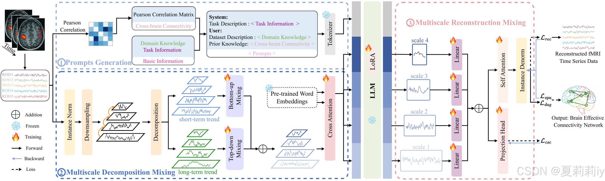
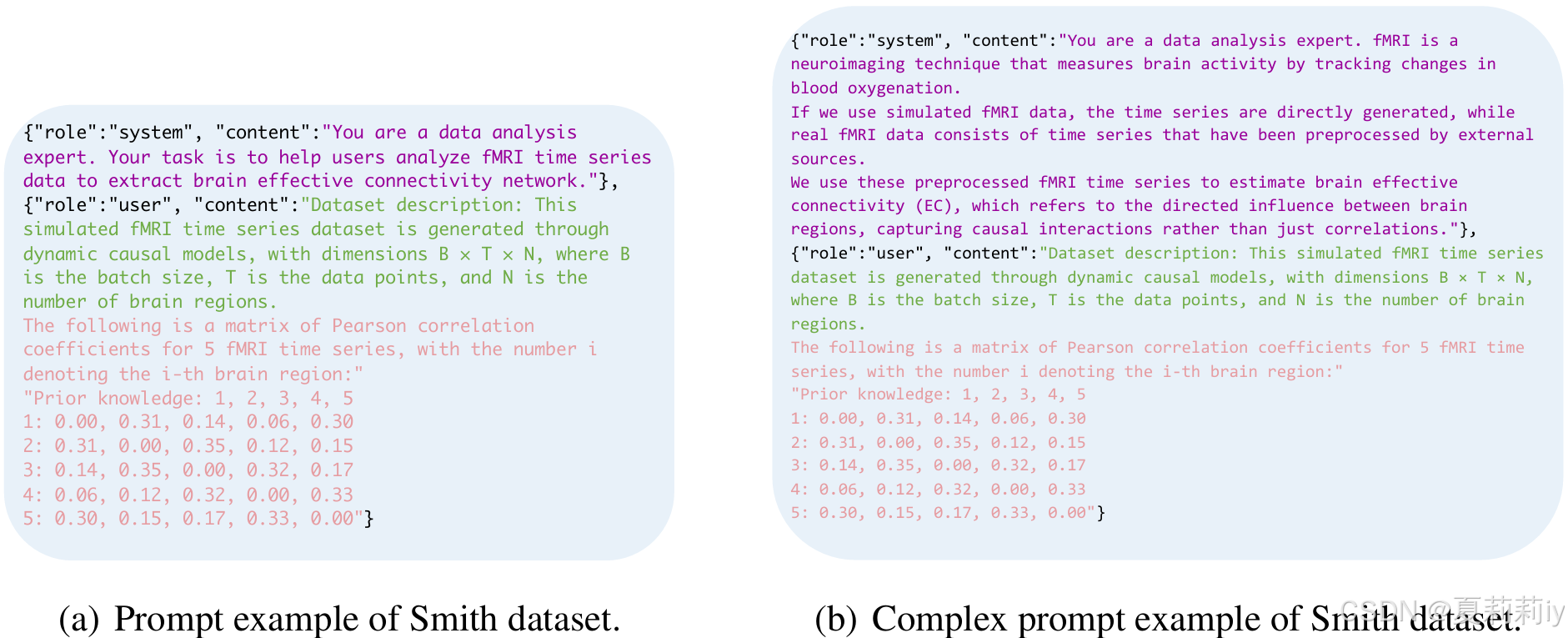
2.5.1. Prompts Generation

        ①提示词：目标描述（任务），数据集描述（如维度），先验知识（皮尔逊相关）

        ②例子：

2.5.2. Multiscale Decomposition Mixing

        ①把fMRI分为有短期趋势（高空间时间分辨率）的和长期趋势（低分辨率）的

（1）Decomposition

        ①按样本把fMRI时间序列进行归一化

        ②持续下采样：

其中是第个尺度的fMRI时间序列

        ③把尺度分解为短期尺度和长期尺度：

（2）Bottom-up Mixing

        ①在短期尺度中，每个分辨率更高（更低尺度）的序列都为分辨率更低的带来额外的信息：

其中是ModernTCN模块：

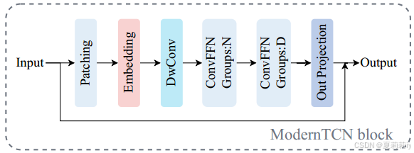
在补丁长度为，步幅为的情况下，补丁总数为

        ②补丁及形状：

        ③对补丁应用一维卷积得到嵌入：

（3）Top-down Mixing

        ①在长期尺度中，每个分辨率更低（更高尺度）的序列都为分辨率更高的带来额外的信息：

（4）Cross Attention

        ①用映射矩阵把LLM语料库中词向量表示从映射到，其中表示词汇量，表示维度

        ②交叉注意力：

其中表示在第个尺度和第个注意力头下的fMRI补丁。就是fMRI而就是词嵌入向量

        ③使用线性层将输出与大模型隐藏层维度对齐：

        ④使用LoRA对大模型进行微调

2.5.3. Multiscale Reconstruction Mixing

        ①大模型输出的进一步被拆分：

        ②将多个尺度的fMRI时间通过线性映射到对齐到:

        ③最终需要重建信号，使用注意力来作为大脑EC

2.5.4. Overall Objective Function

        ①总损失由重建损失，稀疏损失，有向图损失和跨尺度对比损失组成（这是四个？为什么作者说是三个）：

其中有向无环损失：

对比损失：

让相邻尺度的特征更接近而不相邻的远离

        ②对比损失的最大下限：

其中是互信息

2.6. Experiments

2.6.1. Experimental Setups

        ①模拟fMRI数据集：Smith，Sanchez和CDRL

        ②真实fMRI数据集：

Preya Shah, Danielle S Bassett, Laura EM Wisse, John A Detre, Joel M Stein, Paul A Yushkevich, Russell T Shinohara, John B Pluta, Elijah Valenciano, Molly Daffner, et al. Mapping the structural and functional network architecture of the medial temporal lobe using 7t mri. Human Brain Mapping, 39(2):851–865, 2018.

        ③LLM：Llama 3 -8B

        ④所有的实验重复三次

        ⑤设备：Nvidia L20- 48 GB GPU

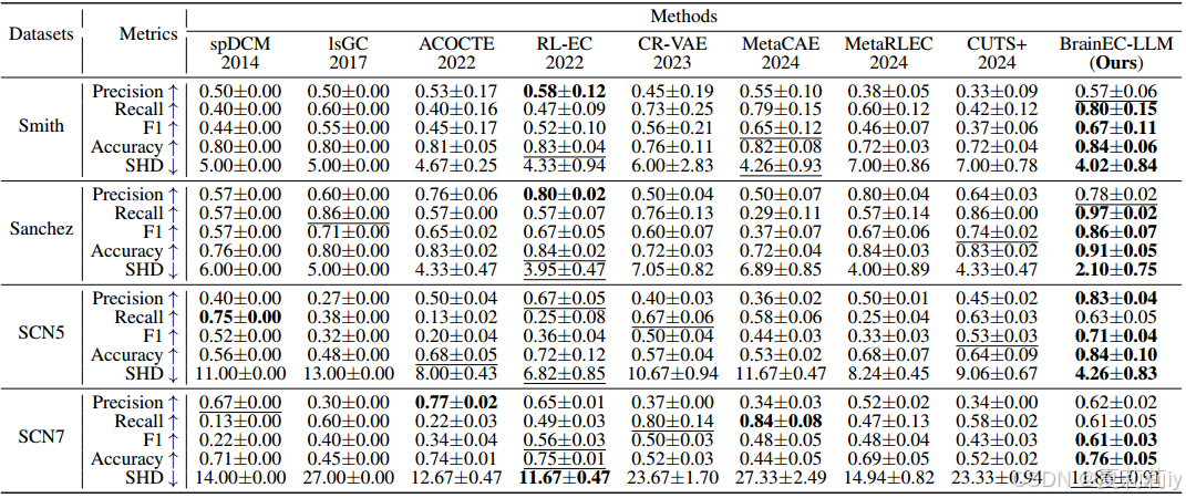
2.6.2. Results on Simulated fMRI Dataset

        ①比较表：

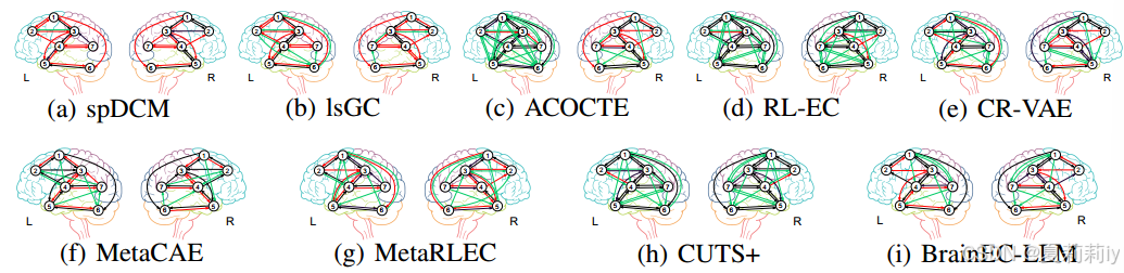
2.6.3. Results on real resting-state fMRI Dataset

        ①可视化EC：

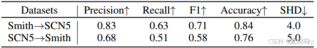
2.6.4. Zero-shot Learning

        ①0样本性能：

2.6.5. Downstream Tasks (Brain Disease Classification using EC networks)

        ①将模型接上SVM作为下游分类器然后分类ABIDE I和ADHD的健康和患病样本：

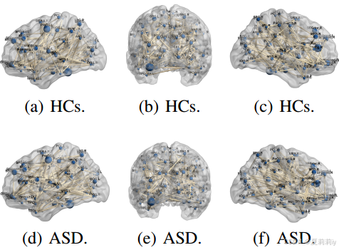
这是前5%有效连接

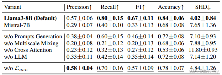
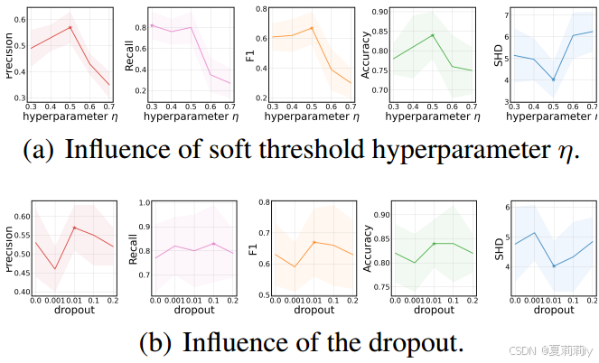
2.6.6. Model Analysis

        ①消融实验：

        ②超参数实验：

2.7. Conclusion

        ~