Matplotlib 简单教程 7：多字图概述

摘要：本文详细介绍了Matplotlib中绘制多图的5种常用方法及其优缺点：1)subplots适合规则网格布局；2)subplot适合逐个创建子图；3)subplot2grid可实现不规则布局；4)GridSpec提供精细布局控制；5)subplot_mosaic支持直观的复杂布局。每种方法都配有完整代码示例，涵盖创建、调整和保存图形的全过程。文章还简要提及了手动创建子图的axes方法，但不推荐

weixin_39204333

1049人浏览 · 2025-11-16 08:45:30

weixin_39204333 · 2025-11-16 08:45:30 发布

1、Matplotlib 多图概述

👏
Matplotlib 库中，可以在 Figure （窗体）上绘制多个子图，常用绘制多图函数有：subplots，subplot，subplot2grid，subplot_mosaic，GridSpec，axes 对比如下：

1.1、subplots

优点：

简洁易用，一次调用可以同时创建多个子图并返回一个包含所有子图的 Figure 对象和一个 Axes 对象的数组，方便进行统一的操作和管理。
自动调整子图之间的间距，使布局更加美观。

缺点：

布局相对较为简单，对于复杂的非规则布局支持有限。

适用情况：

当需要创建规则的网格布局，且不需要非常复杂的子图大小和位置调整时，非常方便。例如创建多个大小相同的子图来展示不同的数据系列。

👏
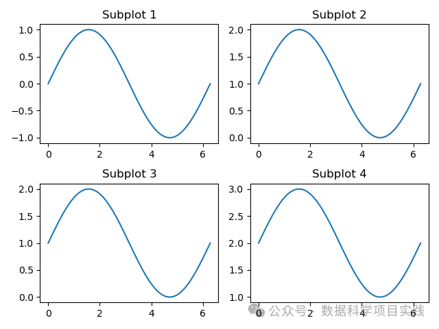
subplots：简洁创建规则网格布局，案例如下：

import matplotlib.pyplot as plt
import numpy as np

fig, axes = plt.subplots(2, 2)

for i in range(2):
    for j in range(2):
        x = np.linspace(0, 2 * np.pi, 100)
        y = np.sin(x) + i + j
        axes[i, j].plot(x, y)
        axes[i, j].set_title(f'Subplot {i * 2 + j + 1}')

# 自动调整化图形布局
plt.tight_layout()

# 保存图形为 PNG 格式
plt.savefig('matplotlib_2024122801.png')

plt.show()

1.2、subplot

优点：

可以逐个创建子图，比较灵活，可以在已有图形的基础上添加新的子图。
对于只需要创建少量子图且逐个处理的情况比较方便。

缺点：

相对繁琐，每次调用只能创建一个子图，如果需要创建多个子图需要多次调用。
不太适合复杂布局。

适用情况：

当需要逐步构建图形，或者只需要创建一两个子图时可以使用。

👏
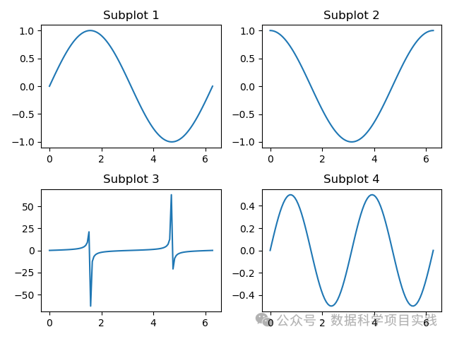
subplot：逐个创建子图，案例如下：

import matplotlib.pyplot as plt
import numpy as np

fig = plt.figure()

ax1 = plt.subplot(221)
x = np.linspace(0, 2 * np.pi, 100)
y = np.sin(x)
ax1.plot(x, y)
ax1.set_title('Subplot 1')

ax2 = plt.subplot(222)
y = np.cos(x)
ax2.plot(x, y)
ax2.set_title('Subplot 2')

ax3 = plt.subplot(223)
y = np.tan(x)
ax3.plot(x, y)
ax3.set_title('Subplot 3')

ax4 = plt.subplot(224)
y = np.sin(x) * np.cos(x)
ax4.plot(x, y)
ax4.set_title('Subplot 4')

# 自动调整化图形布局
plt.tight_layout()

# 保存图形为 PNG 格式
plt.savefig('matplotlib_24122702.png')

plt.show()

1.3、subplot2grid

优点：

可以方便地创建不规则布局的子图，通过指定子图在网格中的起始位置和跨越多行多列的方式来灵活布局。

缺点：

相对于 subplots 来说，语法稍微复杂一些。

适用情况：

当需要创建非规则的子图布局，且需要明确指定子图在网格中的位置和大小跨度时适用。

👏
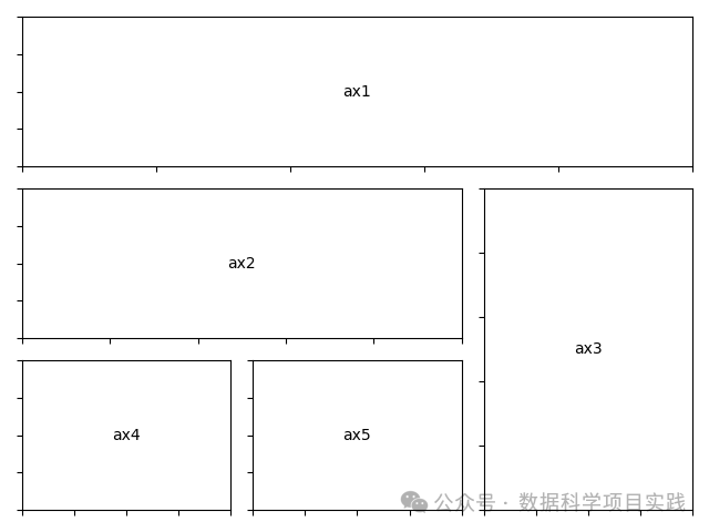
subplot2grid：创建不规则布局，案例如下：

import matplotlib.pyplot as plt

def annotate_axes(fig):
    for i, ax in enumerate(fig.axes):
        ax.text(0.5, 0.5, "ax%d" % (i+1), va="center", ha="center")
        ax.tick_params(labelbottom=False, labelleft=False)

fig = plt.figure()
ax1 = plt.subplot2grid((3, 3), (0, 0), colspan=3)
ax2 = plt.subplot2grid((3, 3), (1, 0), colspan=2)
ax3 = plt.subplot2grid((3, 3), (1, 2), rowspan=2)
ax4 = plt.subplot2grid((3, 3), (2, 0))
ax5 = plt.subplot2grid((3, 3), (2, 1))

annotate_axes(fig)

# 自动调整化图形布局
plt.tight_layout()

# 保存图形为 PNG 格式
plt.savefig('matplotlib_2024122803.png')

plt.show()

def annotate_axes(fig):
    for i, ax in enumerate(fig.axes):
        # 在每个子图的中心位置添加文本
        ax.text(0.5, 0.5, "ax%d" % (i + 1), va="center", ha="center")
        # 设置子图不显示 x 轴和 y 轴的刻度标签
        ax.tick_params(labelbottom=False, labelleft=False)

def annotate_axes(fig):：定义了一个名为annotate_axes的函数，它接受一个matplotlib.figure.Figure对象作为参数。
for i, ax in enumerate(fig.axes):：遍历给定的Figure对象中的所有子图（Axes对象）。enumerate函数在遍历的同时提供了索引i，以便为每个子图添加不同的标注。
ax.text(0.5, 0.5, "ax%d" % (i + 1), va="center", ha="center")：在当前子图的中心位置（坐标(0.5, 0.5)表示在 x 和 y 方向上都处于中间位置）添加文本。文本内容为"ax%d"，其中% (i + 1)会将索引值加 1 后填充到%d的位置，比如第一个子图会显示"ax1"。va="center"表示垂直方向对齐方式为居中，ha="center"表示水平方向对齐方式为居中。
ax.tick_params(labelbottom=False, labelleft=False)：设置当前子图的刻度参数。这里将labelbottom（底部刻度标签显示）设置为False，将labelleft（左侧刻度标签显示）设置为False，即不显示子图的 x 轴底部刻度标签和 y 轴左侧刻度标签。

1.4、GridSpec

优点：

非常灵活，可以创建各种复杂的子图布局，对每个子图的位置和大小有精细的控制。
可以与其他 matplotlib 功能结合使用，如添加标题、坐标轴标签等。

缺点：

语法相对复杂，需要较多的代码来设置布局。

适用情况：

对于复杂的多子图布局，尤其是需要精确控制子图位置和大小的情况非常适用。

👏
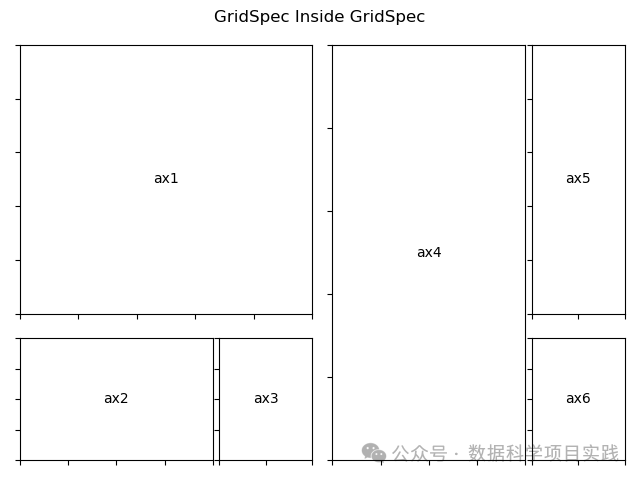
GridSpec：精细控制复杂布局，案例如下：

import matplotlib.pyplot as plt
import matplotlib.gridspec as gridspec

def format_axes(fig):
    for i, ax in enumerate(fig.axes):
        ax.text(0.5, 0.5, "ax%d" % (i+1), va="center", ha="center")
        ax.tick_params(labelbottom=False, labelleft=False)

# gridspec inside gridspec
fig = plt.figure()

gs0 = gridspec.GridSpec(1, 2, figure=fig)

gs00 = gridspec.GridSpecFromSubplotSpec(3, 3, subplot_spec=gs0[0])

ax1 = fig.add_subplot(gs00[:-1, :])
ax2 = fig.add_subplot(gs00[-1, :-1])
ax3 = fig.add_subplot(gs00[-1, -1])

# the following syntax does the same as the GridSpecFromSubplotSpec call above:
gs01 = gs0[1].subgridspec(3, 3)

ax4 = fig.add_subplot(gs01[:, :-1])
ax5 = fig.add_subplot(gs01[:-1, -1])
ax6 = fig.add_subplot(gs01[-1, -1])

plt.suptitle("GridSpec Inside GridSpec")
format_axes(fig)

# 自动调整化图形布局
plt.tight_layout()

# 保存图形为 PNG 格式
plt.savefig('matplotlib_2024122804.png')

plt.show()

def format_axes(fig):
    for i, ax in enumerate(fig.axes):
        ax.text(0.5, 0.5, "ax%d" % (i + 1), va="center", ha="center")
        ax.tick_params(labelbottom=False, labelleft=False)

def format_axes(fig)：定义了一个名为 format_axes 的函数，它接受一个参数 fig，通常这个参数代表一个 matplotlib.figure.Figure 对象。
for i, ax in enumerate(fig.axes)：遍历 fig 对象中的所有子图（轴对象）。enumerate 函数在遍历过程中同时提供了索引 i 和轴对象 ax。
ax.text(0.5, 0.5, "ax%d" % (i + 1), va="center", ha="center")：在每个轴上添加文本。0.5, 0.5 是在轴的坐标系统中，将文本放置在轴的中心位置。"ax%d" % (i + 1) 格式化字符串，用于生成文本内容，例如 ax1、ax2 等。va="center" 和 ha="center" 分别表示垂直对齐和水平对齐方式为居中。
ax.tick_params(labelbottom=False, labelleft=False)：设置轴的刻度标签显示。这里将底部和左侧的刻度标签设置为不显示。这样可以在不需要显示刻度标签的情况下清理子图的外观。

1.5、subplot_mosaic

优点：

使用类似字典的布局描述方式，非常直观，易于理解和设置复杂的布局。
可以方便地通过名称访问子图，提高代码的可读性。

缺点：

相对较新，可能在一些旧版本的环境中不可用。

适用情况：

当需要创建复杂的非规则布局，并且希望以一种更直观的方式进行布局设置时适用。

👏
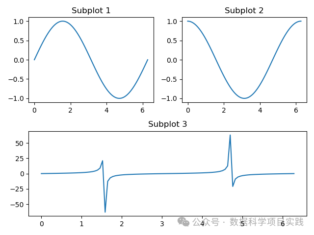
subplot_mosaic： 直观创建复杂布局，案例如下：

import matplotlib.pyplot as plt
import numpy as np

fig, ax_dict = plt.subplot_mosaic(
    [['top_left', 'top_right']
    ,['bottom', 'bottom']]
    )

x = np.linspace(0, 2 * np.pi, 100)
y_sin = np.sin(x)
y_cos = np.cos(x)
y_tan = np.tan(x)

ax_dict['top_left'].plot(x, y_sin)
ax_dict['top_left'].set_title('Subplot 1')

ax_dict['top_right'].plot(x, y_cos)
ax_dict['top_right'].set_title('Subplot 2')

ax_dict['bottom'].plot(x, y_tan)
ax_dict['bottom'].set_title('Subplot 3')

# 自动调整化图形布局
plt.tight_layout()

# 保存图形为 PNG 格式
plt.savefig('matplotlib_2024122805.png')

plt.show()

1.6、axes

👏
严格来说，axes 不是专门用于创建多图的函数，但可以通过手动设置坐标轴位置来创建多个子图。

优点：

非常灵活，可以完全自定义子图的位置和大小。

缺点：

需要手动计算和设置坐标轴位置，非常繁琐，容易出错。

适用情况：

在一些非常特殊的情况下，需要极其精细地控制子图位置和大小，且其他方法无法满足需求时可以考虑使用，但一般不推荐。

👏
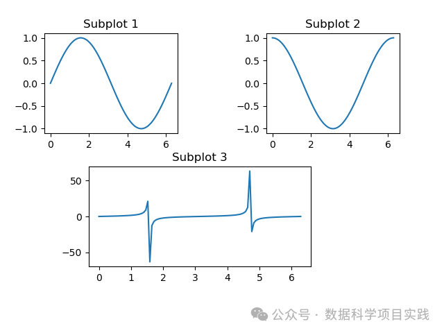
axes： 手动创建子图，案例如下：

import matplotlib.pyplot as plt
import numpy as np

fig = plt.figure()

ax1 = fig.add_axes([0.1, 0.6, 0.3, 0.3])
x = np.linspace(0, 2 * np.pi, 100)
y = np.sin(x)
ax1.plot(x, y)
ax1.set_title('Subplot 1')

ax2 = fig.add_axes([0.6, 0.6, 0.3, 0.3])
y = np.cos(x)
ax2.plot(x, y)
ax2.set_title('Subplot 2')

ax3 = fig.add_axes([0.2, 0.2, 0.5, 0.3])
y = np.tan(x)
ax3.plot(x, y)
ax3.set_title('Subplot 3')

# 自动调整化图形布局
plt.tight_layout()

# 保存图形为 PNG 格式
plt.savefig('matplotlib_2024122806.png')

plt.show()