机器学习-准备 scikit-learn-Orange安装
一、scikit-learn引导1.1scikit-learn 是什么面向python免费机器学习库建立在Numpy、Scipy、和 scikit-learn 模块之上包含分类、回归、聚类算法 比如:SVM,随机森林,K-mean等包含降维、模型筛选、预处理算法1.2 scikit-learn 安装推荐Anaconda 已经封装了 scikit-lear...
·
一、scikit-learn引导
1.1 scikit-learn 是什么
面向python免费机器学习库
建立在Numpy、Scipy、和 scikit-learn 模块之上
包含分类、回归、聚类算法 比如:SVM,随机森林,K-mean等
包含降维、模型筛选、预处理算法
1.2 scikit-learn 安装
推荐Anaconda 已经封装了 scikit-learn
Anaconda 查询包信息:
    conda list|grep matplotlib

通过 pip 安装
    由于 scikit-learn 建立在Numpy、Scipy 模块之上,必须先安装这两个
    pip install -U numpy scipy scikit-learn
1.3 scikit-learn API
1.3.1 sklearn常用数据集一览
类型 获取方式 自带小数据集 sklearn.datasets.load_ 在线下载的数据集 sklearn.datasets.fetch_ 计算机生成的数据集 sklearn.datasets.make_ svmlight/libsvm格式的数据集 sklearn.datasets.load_svmlight_file(…) mldata.org在线下在数据集 sklearn.datasets.fetch_mldata 1.3.2 sklearn自带的小数据集
自带的小数据集
名称 数据包调用方式 适用算法 鸢尾花数据集 load_iris() 分类 乳腺癌数据集 load_bread_cancer() 二分类任务 手写数字数据集 load_digits() 分类 糖尿病数据集 load_diabetes() 回归 波士顿房价数据集 load_boston() 回归 体能训练数据集 load_linnerud() 多变量回归 1.3.2 iris(鸢尾花)数据集的查看
iris包含150个样本,对应数据集的每行数据。每行数据包含每个样本的四个特征和样本的类别信息,所以iris数据集是一个150行5列的二维表。
每个样本包含了花萼长度、花萼宽度、花瓣长度、花瓣宽度四个特征(前4列,单位cm)和品种信息,即目标属性(第5列,也叫target或label)。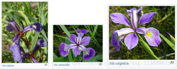
from sklearn import datasets
import matplotlib.pyplot as plt
from sklearn.datasets import load_iris

iris=load_iris()        #加载数据集
iris.keys()

输出: dict_keys(['target', 'DESCR', 'data', 'target_names', 'feature_names'])

n_samples,n_features=iris.data.shape
print("Number of sample:",n_samples)
print("Number of feature",n_features)
print(iris.data[0])     #第一个样例
print(iris.data.shape)
print(iris.target.shape)
print(iris.target)

依次输出
: Number of sample: 150
: Number of feature 4
: [ 5.1 3.5 1.4 0.2]    #第一个样例输出
: (150, 4)
: (150,)
: [0 0 0 0 0 0 0 0 0 0 0 0 0 0 0 0 0 0 0 0 0 0 0 0 0 0 0 0 0 0 0 0 0 0 0 0 0
    0 0 0 0 0 0 0 0 0 0 0 0 0 1 1 1 1 1 1 1 1 1 1 1 1 1 1 1 1 1 1 1 1 1 1 1 1
    1 1 1 1 1 1 1 1 1 1 1 1 1 1 1 1 1 1 1 1 1 1 1 1 1 1 2 2 2 2 2 2 2 2 2 2 2
    2 2 2 2 2 2 2 2 2 2 2 2 2 2 2 2 2 2 2 2 2 2 2 2 2 2 2 2 2 2 2 2 2 2 2 2 2
    2 2]
iris=datasets.load_iris() x_index=3 color=['blue','red','green'] for label,color in zip(range(len(iris.target_names)),color): plt.hist(iris.data[iris.target==label,x_index], label=iris.target_names[label], color=color) plt.xlabel(iris.feature_names[x_index]) plt.legend(loc='upper right') plt.show()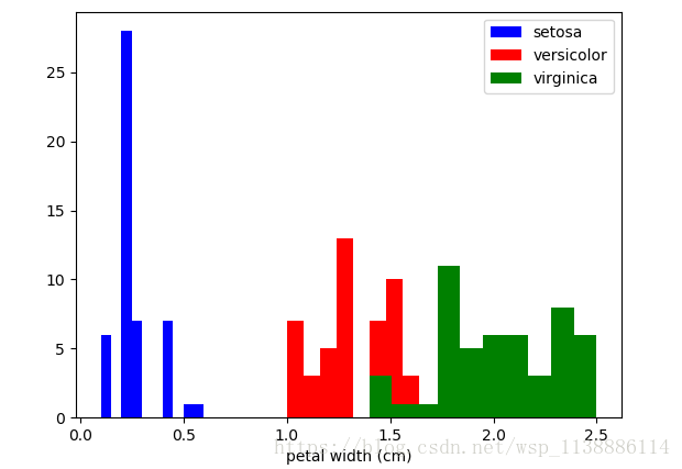
iris=datasets.load_iris()
x_index=0
y_index=1
colors=['blue','red','green']
for label,color in zip(range(len(iris.target_names)),colors):
    plt.scatter(iris.data[iris.target==label,x_index],
    iris.data[iris.target==label,y_index],
    label=iris.target_names[label],
    c=color)
plt.xlabel(iris.feature_names[x_index])
plt.ylabel(iris.feature_names[y_index])
plt.legend(loc='upper left')
plt.show()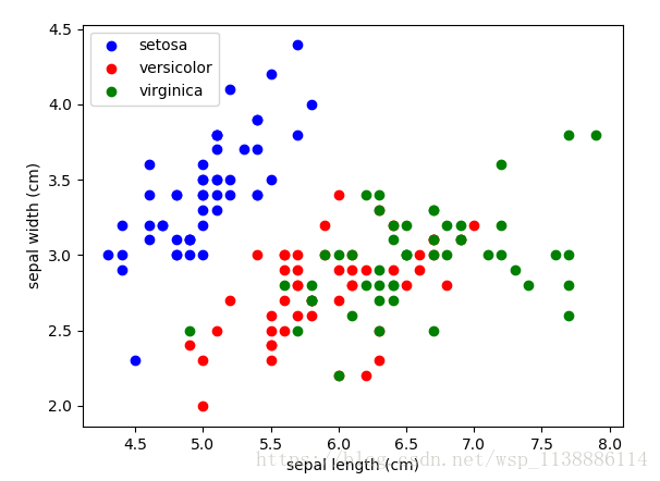
1.4 scikit-learn 三个主要概念
估计器 Estimator :用于分类,聚类,回归
    主要函数:
        fit():训练算法,设置内部参数,接受训练集和内别两个参数
        predict(): 预测测试集类别,参数为测试集
    大多数 scikit-learn 估计器接收和输出数据格式均为numpy或类似格式
        scikit-learn之估计器运行流程
                转换器 Transformer:用于数据预处理,数据转换

流水线 Pipeline: 组合数据挖掘,便于再次使用
    sklearn.pipeline 包
    流水线功能:
        跟踪记录各步骤的操作(以便重现实验结果)
        对各步骤进行封装
        确保代码复杂程度不至于超出掌控范围

    基本使用方法
        流水线输入 一连串数据挖掘步骤
        其中最后一步必须是预估器 前几步是转换器
        输入的数据集经过转换器处理后,上一步输出->下一步输入。。。->估计器,对数据进行分类
        每一步都有元组('名称','步骤')来表示
from sklearn import datasets
from sklearn.model_selection import train_test_split
from sklearn.neighbors import KNeighborsClassfier
iris_x = iris.data
iris_y = iris.target
x_train,x_test,y_train,y_test = train_test_split(iris_x,iris_y,test_size = 0.3)

model = KNeighborsClassfier()
model.fit(x_train,y_train)
print(model.predict(x_test))
print(y_test)
二、Orange 与可视化机器学习
2.1 Orange 简介
老司机可作为Python模块2.2 Orange 安装
Orange 已经完全转到python3 项目主页请点击
▶ 安装步骤(
python3.x环境):在 Anaconda Prompt 下执行: conda create --name Py35_Orange3 python=3.5▶ 激活环境:
activate Py35_Orange3          #for windows
source activate Py35_Orange3   #for Linux/MacOS
▶ 安装 orange3
pip install orange3▶ 验证是否安装成功
>>> import Orange
>>> Orange.version.version
Orange扩展包-关联
在 Orange3 中,关联规则算法在 add-on 包中
项目主页:https://pypi.python.org/pypi/Orange3-Associate
通过 pip 安装
pip install Orange3-Associate
Orange扩展包-协同过滤
在 Orange3 中,协同过滤算法在 add-on 包中
项目主页:https://github.com/mstrazar/orange
通过 pip 安装
pip install Orange3-recommenddation2.3 Orange 使用方式
使用方式 1 –脚本
from orangecontrib.associate.fpgrowth import *  #关联
T = [[1,3,4],
    [2,3,5],
    [1,2,3,5],
    [2,5]]
itemset = dict(frequent_itemsets(T,2))
itemset
rules = [(P,Q,supp,conf)
          for P,Q,supp,conf in association_rules(itemsets,.8)if len(Q)==1]
(rules)
使用方式 2 图形界面
source activate python35
orange-canvas&
2.4 Orange 功能结构–数据准备与预处理
Data
visualize
model
evaluate
三、Xgboost 简介
Xgboost 是大规模并行boosted tree 工具
安装 Xgboost 的python 版需要Numpy,Scipy等数值计算库,

Xgboost 安装--Linux
    升级包版本
    $ conda updata -all
    安装
    pip install xgboost
    测试
    $python

Xgboost 安装-windows
python3.5及以上版本,基于anaconda
http://www.lfd.uci.edu/~gohlke/pythonlibs/#xgboost 在以上网站找对应版本
安装(install后面为下载保存位置+下载版本)
pip install xgboost-0.6-cp35-cp35m-win_amd64.whl
四、 sklearn 主要算法调用及比较
import numpy as np
import matplotlib.pyplot as plt
from matplotlib.colors import ListedColormap
#from sklearn.model_selection import train_test_split #废弃!!
from sklearn.cross_validation import train_test_split
from sklearn.preprocessing import StandardScaler
from sklearn.datasets import make_moons, make_circles, make_classification
from sklearn.neural_network import BernoulliRBM
from sklearn.neighbors import KNeighborsClassifier
from sklearn.svm import SVC
from sklearn.gaussian_process import GaussianProcess
from sklearn.tree import DecisionTreeClassifier
from sklearn.ensemble import RandomForestClassifier, AdaBoostClassifier
from sklearn.naive_bayes import GaussianNB
from sklearn.discriminant_analysis import QuadraticDiscriminantAnalysis

h = .02  # step size in the mesh

names = ["Nearest Neighbors", "Linear SVM", "RBF SVM",
         "Decision Tree", "Random Forest", "AdaBoost",
         "Naive Bayes", "QDA", "Gaussian Process","Neural Net", ]

classifiers = [
    KNeighborsClassifier(3),
    SVC(kernel="linear", C=0.025),
    SVC(gamma=2, C=1),
    DecisionTreeClassifier(max_depth=5),
    RandomForestClassifier(max_depth=5, n_estimators=10, max_features=1),
    AdaBoostClassifier(),
    GaussianNB(),
    QuadraticDiscriminantAnalysis(),
    #GaussianProcess(),
    #BernoulliRBM(),
    ]

X, y = make_classification(n_features=2, n_redundant=0, n_informative=2,
                           random_state=1, n_clusters_per_class=1)
rng = np.random.RandomState(2)
X += 2 * rng.uniform(size=X.shape)
linearly_separable = (X, y)

datasets = [make_moons(noise=0.3, random_state=0),
            make_circles(noise=0.2, factor=0.5, random_state=1),
            linearly_separable
            ]

figure = plt.figure(figsize=(27, 9))
i = 1
# iterate over datasets
for ds_cnt, ds in enumerate(datasets):
    # preprocess dataset, split into training and test part
    X, y = ds
    X = StandardScaler().fit_transform(X)
    X_train, X_test, y_train, y_test = \
        train_test_split(X, y, test_size=.4, random_state=42)

    x_min, x_max = X[:, 0].min() - .5, X[:, 0].max() + .5
    y_min, y_max = X[:, 1].min() - .5, X[:, 1].max() + .5
    xx, yy = np.meshgrid(np.arange(x_min, x_max, h),
                         np.arange(y_min, y_max, h))

    # just plot the dataset first
    cm = plt.cm.RdBu
    cm_bright = ListedColormap(['#FF0000', '#0000FF'])
    ax = plt.subplot(len(datasets), len(classifiers) + 1, i)
    if ds_cnt == 0:
        ax.set_title("Input data")
    # Plot the training points
    ax.scatter(X_train[:, 0], X_train[:, 1], c=y_train, cmap=cm_bright)
    # and testing points
    ax.scatter(X_test[:, 0], X_test[:, 1], c=y_test, cmap=cm_bright, alpha=0.6)
    ax.set_xlim(xx.min(), xx.max())
    ax.set_ylim(yy.min(), yy.max())
    ax.set_xticks(())
    ax.set_yticks(())
    i += 1

    # iterate over classifiers
    for name, clf in zip(names, classifiers):
        ax = plt.subplot(len(datasets), len(classifiers) + 1, i)
        clf.fit(X_train, y_train)
        score = clf.score(X_test, y_test)

        # Plot the decision boundary. For that, we will assign a color to each
        # point in the mesh [x_min, m_max]x[y_min, y_max].
        if hasattr(clf, "decision_function"):
            Z = clf.decision_function(np.c_[xx.ravel(), yy.ravel()])
        else:
            Z = clf.predict_proba(np.c_[xx.ravel(), yy.ravel()])[:, 1]

        # Put the result into a color plot
        Z = Z.reshape(xx.shape)
        ax.contourf(xx, yy, Z, cmap=cm, alpha=.8)

        # Plot also the training points
        ax.scatter(X_train[:, 0], X_train[:, 1], c=y_train, cmap=cm_bright)
        # and testing points
        ax.scatter(X_test[:, 0], X_test[:, 1], c=y_test, cmap=cm_bright,
                   alpha=0.6)

        ax.set_xlim(xx.min(), xx.max())
        ax.set_ylim(yy.min(), yy.max())
        ax.set_xticks(())
        ax.set_yticks(())
        if ds_cnt == 0:
            ax.set_title(name)
        ax.text(xx.max() - .3, yy.min() + .3, ('%.2f' % score).lstrip('0'),
                size=15, horizontalalignment='right')
        i += 1

plt.tight_layout()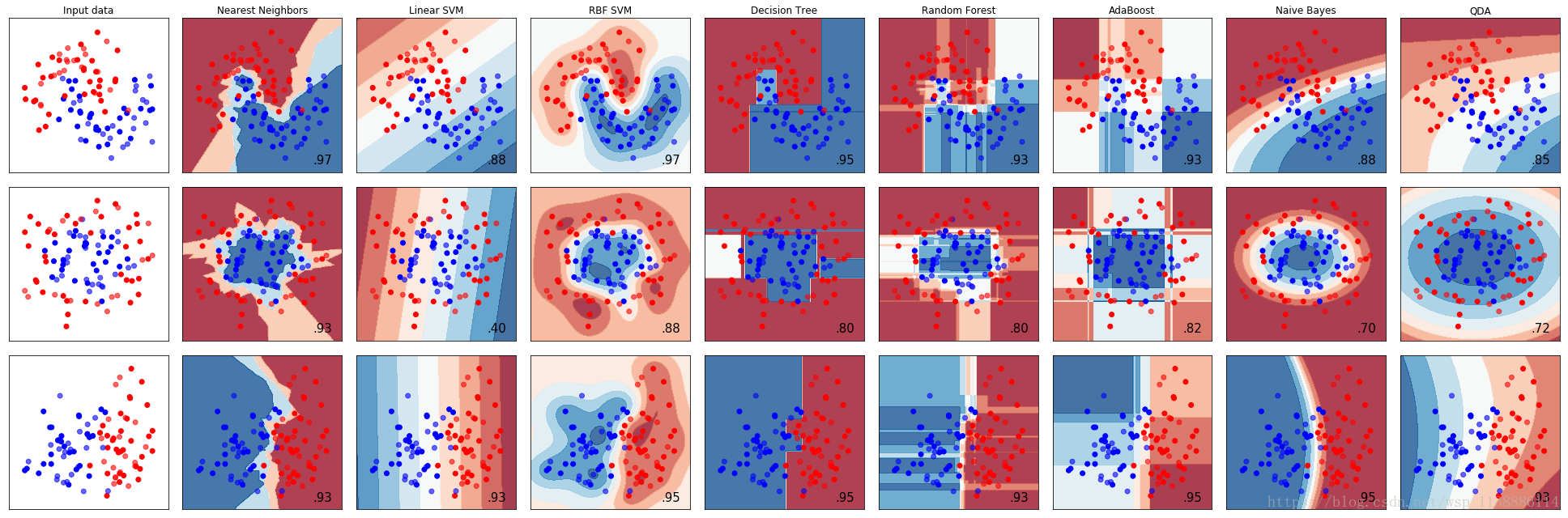

有“AI”的1024 = 2048,欢迎大家加入2048 AI社区
更多推荐
 4
4 0
0- 0


 已为社区贡献70条内容

所有评论(0)