5、目标检测:损失函数
一、损失函数分类及原理L1、L2 LossSmooth-L1-LossFocal-Loss二、损失函数在 TF 中的实现# smooth-l1-lossdef bbox_ohem_smooth_L1_loss(bbox_pred, bbox_target, label):sigma = tf.constant(1.0)threshold = 1.0 / (...
一、目标检测中的分类损失
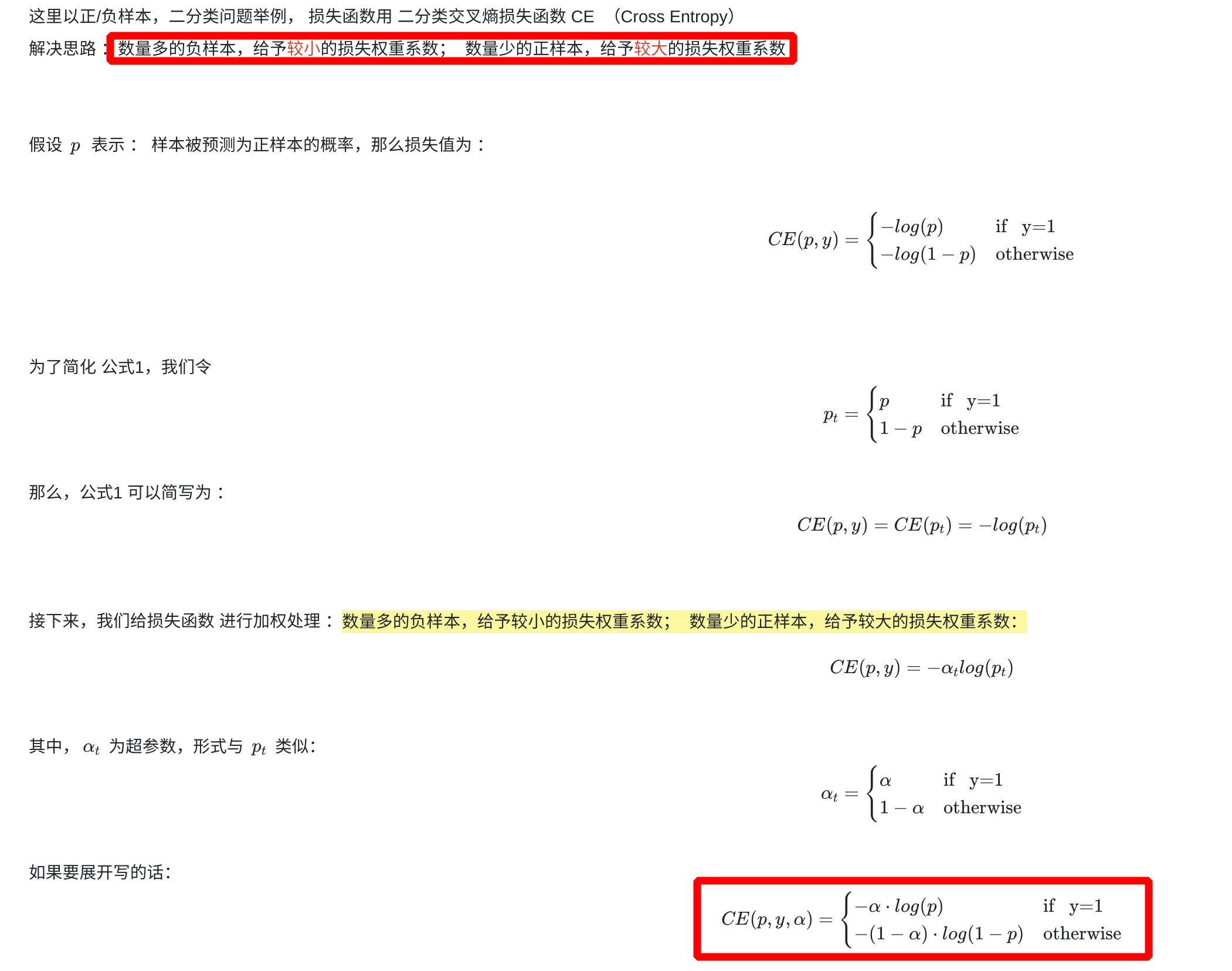
1.1、cross_entropy_loss
-
softmax_cross_entropy_loss(多分类)以及sigmoid_cross_entropy_loss(二分类)可参考博客: TensorFLow 中的损失函数 -
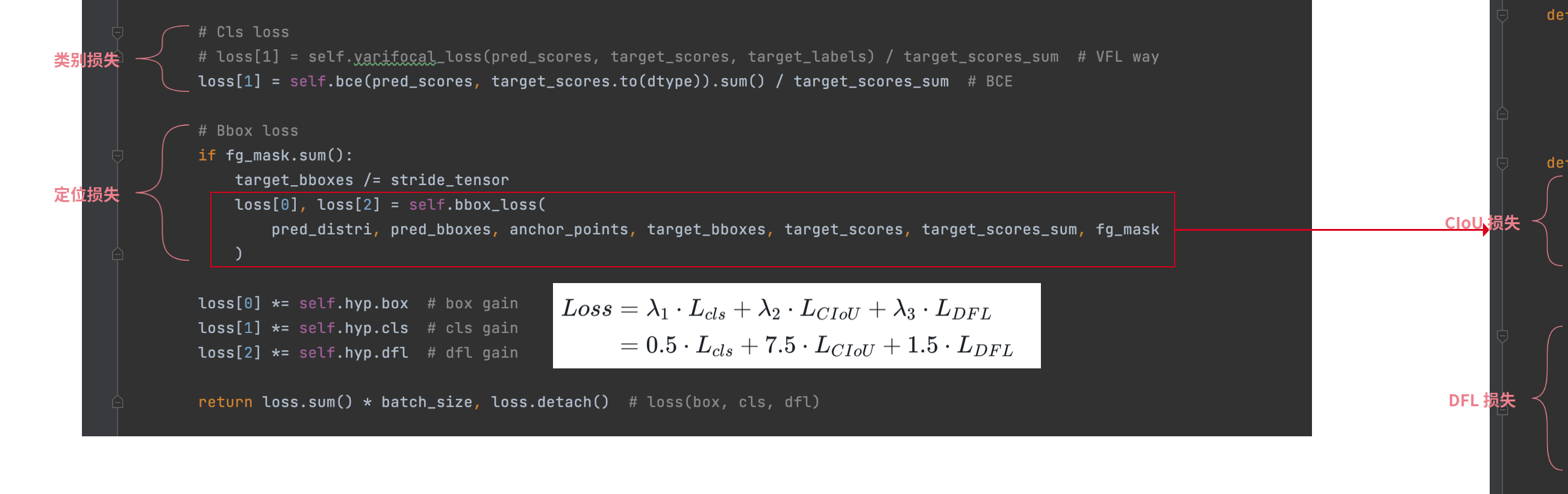
YOLOv8 中的二分类交叉熵损失函数:
- 16 为
batch size - 8400 为
anchor point的数量 - 80 为类别数量,
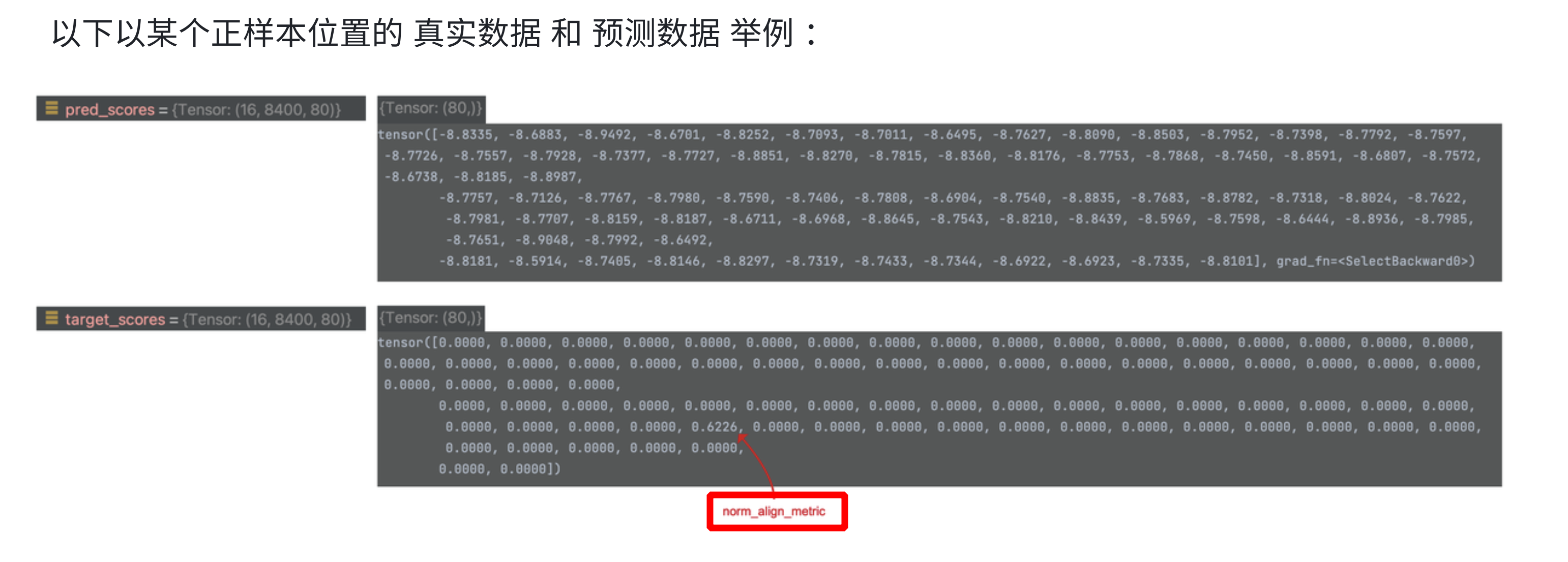
pred_scores中的值为网络预测的logits,未经过 sigmoid;target_scores 中的 GT 值为正样本的norm_align_metric值(结合了 CIoU 和 score 后对齐的值,取值范围是0-1,不是原来的1) - 注意:最终的值还要除以
target_score_sum做归一化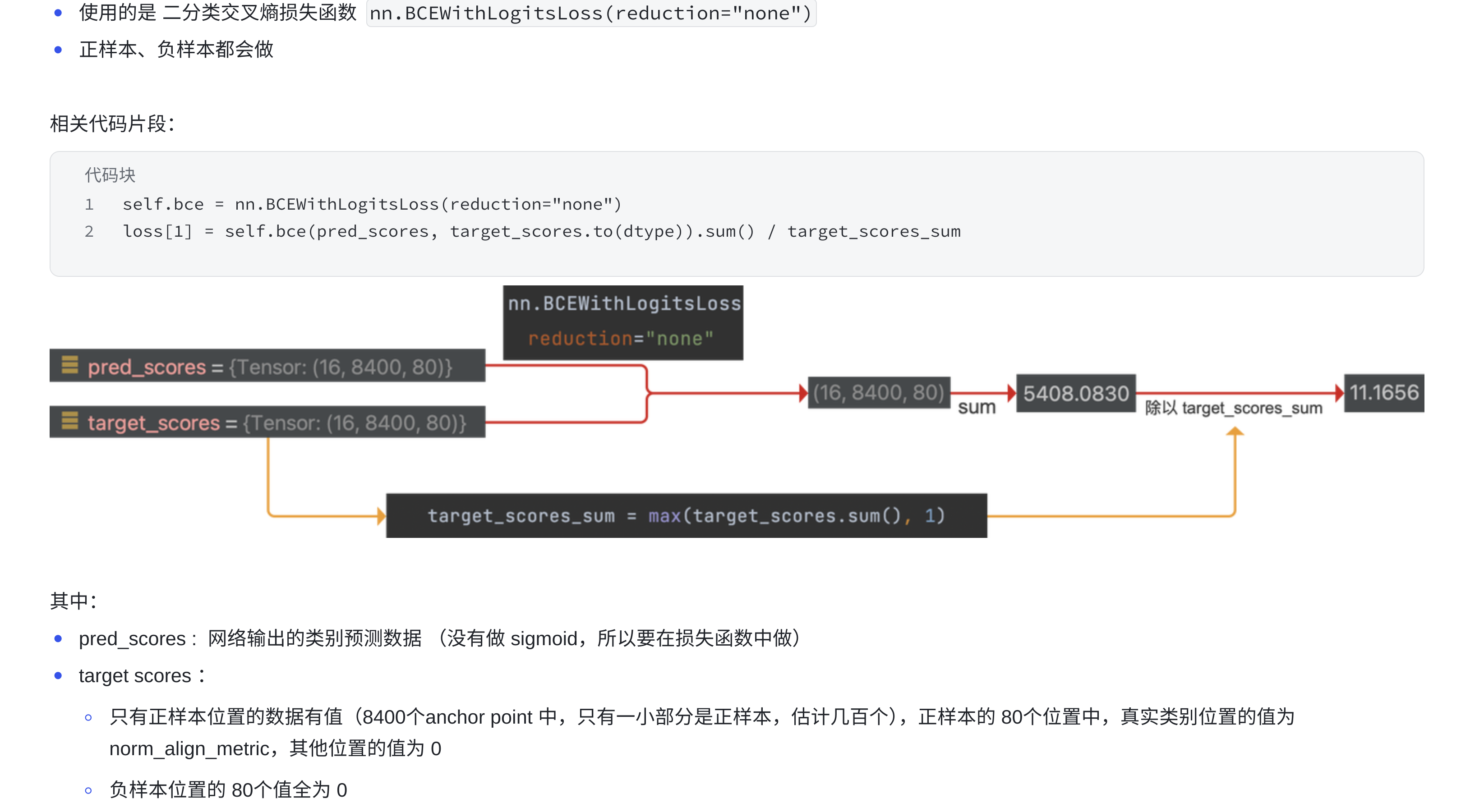
- 16 为
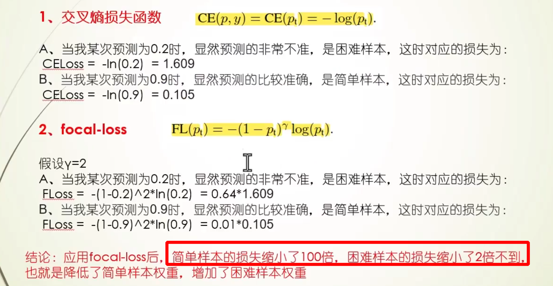
1.2、focal_loss

-
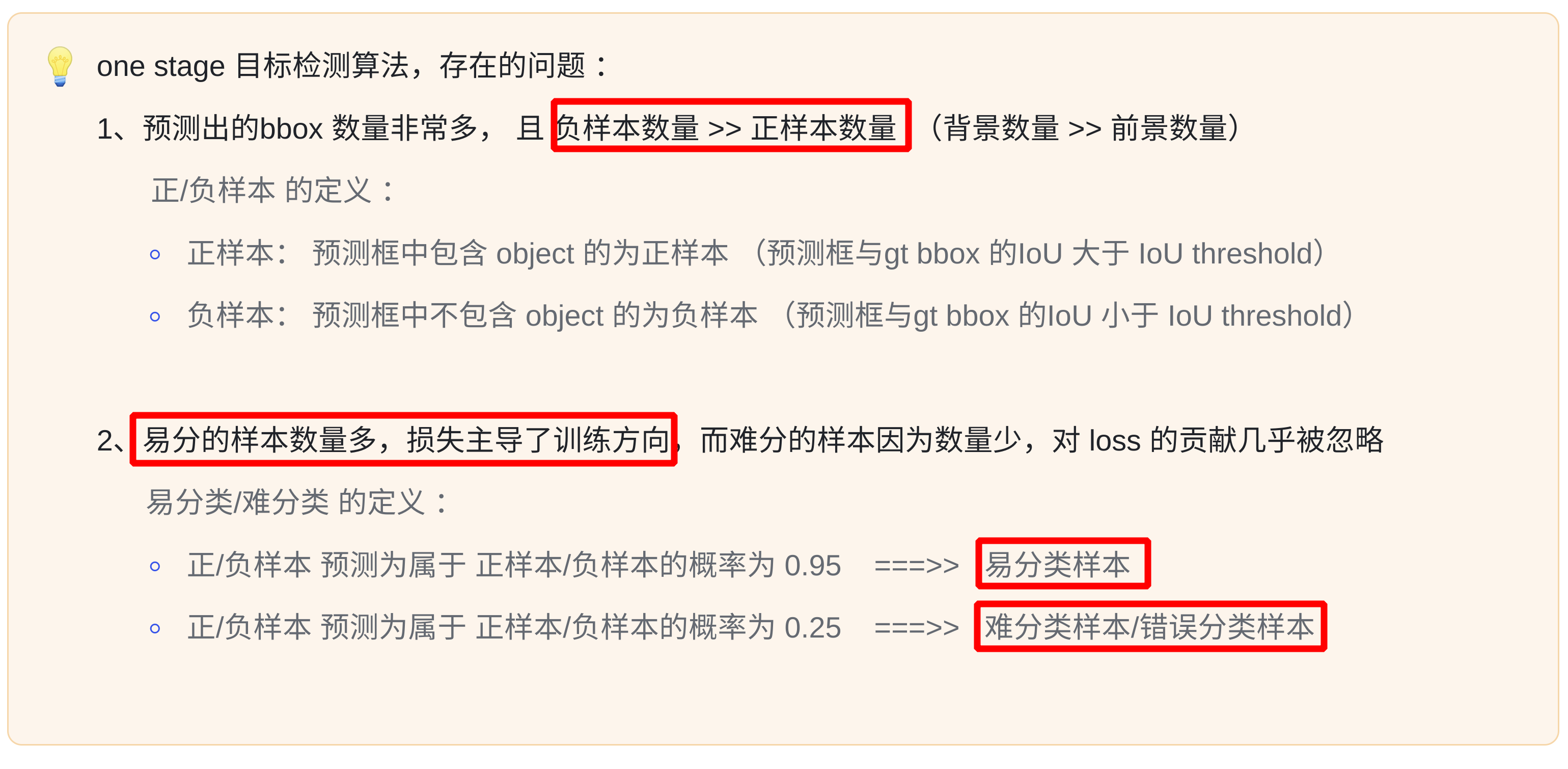
Focal loss(全局视角):- 思想:用一个权重条件函数(置信度的角度)去降低
易分样本(inference 中概率得分较大的)对损失的贡献(得分较大时降低其损失值,使得简单样本对损失的影响更小) - 使用场景:解决 one-stage 的目标检测中背景样本和前景样本的不平衡问题
- 调参经验:
- 降低 neg_overlap 的值(eg:0.3),ignore 一部分(0.3~0.5)label noise sample(1、标签打错了,2、困难样本)
- fine-tuning 时用:先在原始 loss 上预训练几个 epoch,然后再换成 focal loss
- 增加 anchor 数量、batch_size 等
- 分类 loss 选择
LOGISTIC(二分类)而不是SOFTMAX(多分类)
- 思想:用一个权重条件函数(置信度的角度)去降低
-
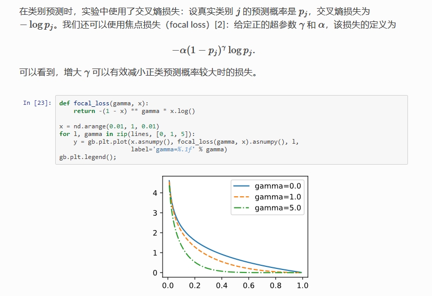
Focal loss 公式:-
多分类公式: F L ( p t ) = − α t ( 1 − p t ) γ l o g ( p t ) FL(p_t) = -\alpha_t(1 - p_t)^{\gamma} log(p_t) FL(pt)=−αt(1−pt)γlog(pt)
- α t \alpha_t αt:控制类别间的权重比例,例如二分类中的 0.25(
pos:neg = 1:3) - γ \gamma γ:控制 loss 衰减的快慢,结合 ( 1 − p t ) (1 - p_t) (1−pt) 解决难易样本不平衡的问题
- 参数组合:论文中效果较好的为 α = 0.25 , γ = 2.0 \alpha = 0.25,\gamma=2.0 α=0.25,γ=2.0
- α t \alpha_t αt:控制类别间的权重比例,例如二分类中的 0.25(
-
α \alpha α:解决正负样本数量不均衡的问题
-
( 1 − p t ) γ (1 - p_t)^{\gamma} (1−pt)γ:降低
易分样本(inference 中概率得分较大的)对损失的贡献,相对增加难分样本对损失的贡献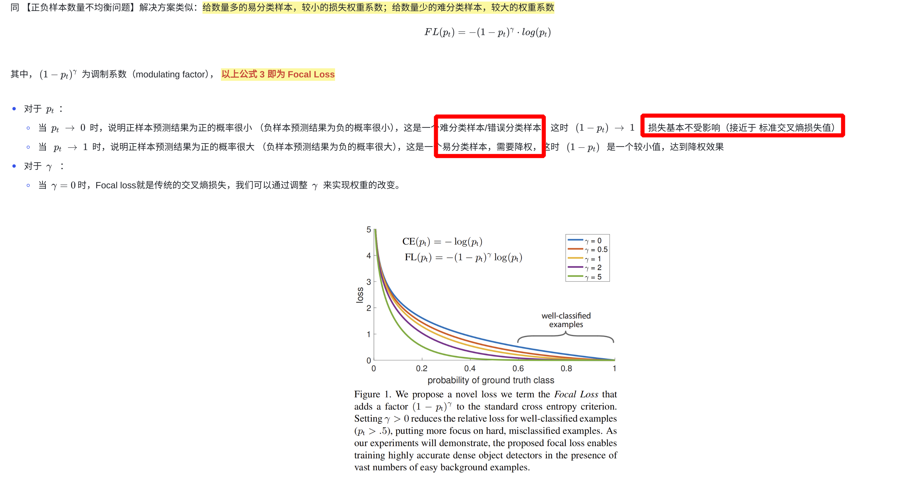
-
pytorch 代码实现:
import torch import torch.nn as nn import torch.nn.functional as F class Focal_Loss(nn.Module): def __init__(self, alpha, gamma=2, logits=True): super(Focal_Loss, self).__init__() self.alpha = alpha # 损失权重,长度等于类别数的向量 self.gamma = gamma self.logits = logits self.class_num = len(alpha) def forward(self, preds, labels): """ preds: size=(n, m), n个样本, 以及对应的预测出的m个类别的概率 labels: size=(n), n个样本的真实类别 """ if not self.logits: preds = F.softmax(preds, dim=-1) # 将类别序号转换成 onehot 的形式 labels_onehot = F.one_hot(labels, num_classes=self.class_num) eps = 1e-8 floss = -1 * self.alpha * torch.pow((1 - preds), self.gamma) * torch.log(preds + eps) * labels_onehot return torch.mean(torch.sum(floss, dim=1)) if __name__ == '__main__': preds = torch.randn(5, 10) # 5个样本对应的预测出10个类别的概率 labels = torch.randint(0, 10, (5,)) # 5个样本的真实类别,共10个类别,序号从 0~9 weights = torch.randn(10) # 10个类别的损失权重 focal_loss = Focal_Loss(alpha=weights, logits=False) loss = focal_loss(preds, labels) print(loss) -
-
caffe 中的实现,参见 https://github.com/chuanqi305/FocalLoss
layer { name: "mbox_loss" type: "MultiBoxFocalLoss" // change the type bottom: "mbox_loc" bottom: "mbox_conf" bottom: "mbox_priorbox" bottom: "label" top: "mbox_loss" include { phase: TRAIN } propagate_down: true propagate_down: true propagate_down: false propagate_down: false loss_param { normalization: VALID } focal_loss_param { alpha: 0.25 gamma: 2.0 } multibox_loss_param { loc_loss_type: SMOOTH_L1 conf_loss_type: SOFTMAX // 二分类的时候换成 LOGISTIC 效果会好些 loc_weight: 1.0 num_classes: 21 share_location: true match_type: PER_PREDICTION overlap_threshold: 0.5 use_prior_for_matching: true background_label_id: 0 use_difficult_gt: true neg_pos_ratio: 3.0 neg_overlap: 0.5 code_type: CENTER_SIZE ignore_cross_boundary_bbox: false mining_type: NONE #do not use OHEM } } -
one-stage detector 精度比不上 two-stage detector 的原因:
- 正负样本比例极度不平衡(一般大约 10000:1),且绝大部分负样本都是 easy example
gradient 被 easy example dominant,往往这些 easy example 虽然 loss 很低,但由于数量众多,对于 loss 依旧有很大贡献,从而导致收敛到不够好的一个结果- 若分类器无脑地把所有 bbox 统一归类为 background,accuracy 也可以刷得很高。于是乎,分类器的训练就失败了。分类器训练失败,检测精度自然就低了
- two-stage 系有 RPN 罩着,RPN 会对 anchor 进行简单的二分类,anchor box 数量降低很多(1~2k),后续再使用 OHEM+按 class 比例 sample(eg:1:3),即可很好的进行训练
-
OHEM+按 class 比例 sample 原理:
- each example is scored by its loss, non-maximum suppression (nms) is then applied, and a minibatch is constructed with the highest-loss examples(
enforce a 1:3 ratio) - 相比 Focal loss,OHEM 算法虽然增加了错分类样本的权重,但是 OHEM 算法忽略了容易分类的样本,focal loss 相当于全局视角,把所有情况都考虑进去了
- each example is scored by its loss, non-maximum suppression (nms) is then applied, and a minibatch is constructed with the highest-loss examples(
1.3、信息量、熵、交叉熵、相对熵(KL 散度)、交叉熵损失函数
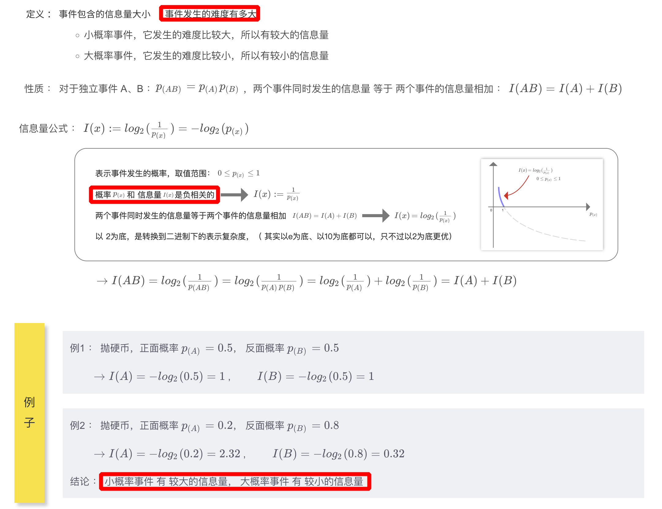
1.3.1、信息量
- 信息量表示为事件发生的难度,与事件发生的概率是
负相关的 - 之所以加上对数(
对数相乘可以转换为相加),是因为要实现两个事件同时发生的信息量等于两个事件信息量相加
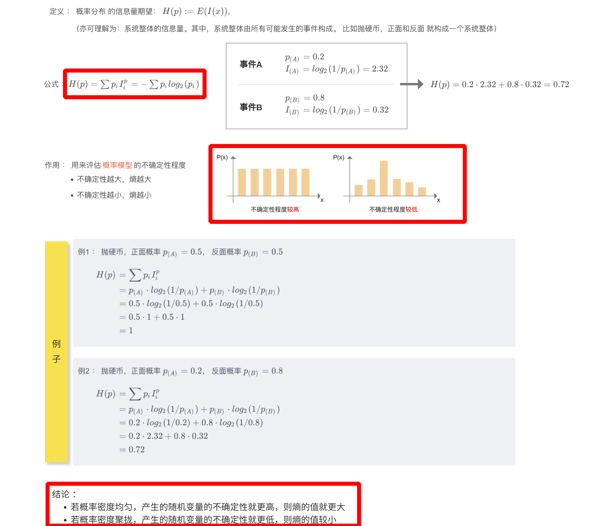
1.3.2、熵
- 熵定义为 概率分布的信息量期望,可以用来评估概率模型的不确定程度,熵越大,不确定性越大,熵越小,不确定性越小
- 熵又包含:交叉熵和相对熵(KL 散度)
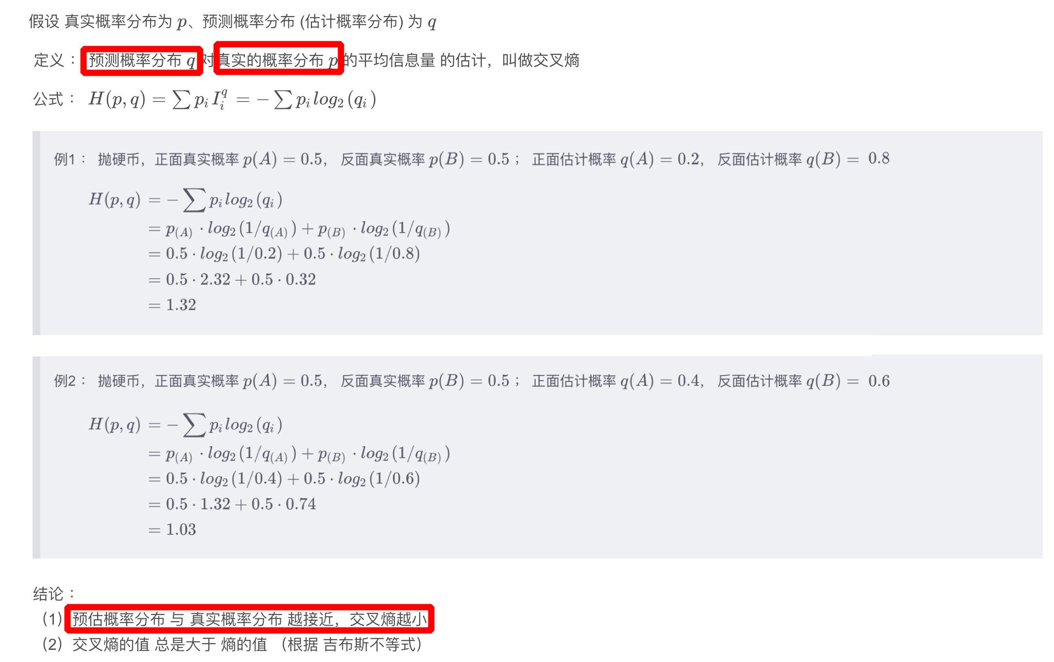
1.3.3、交叉熵
- 交叉熵:
- 在熵的基础上,真实概率分布
p保持不变,而信息量换成预测概率分布的信息量 I q I^q Iq - 预测概率分布与真实概率分布越接近,交叉熵越小
- 在熵的基础上,真实概率分布
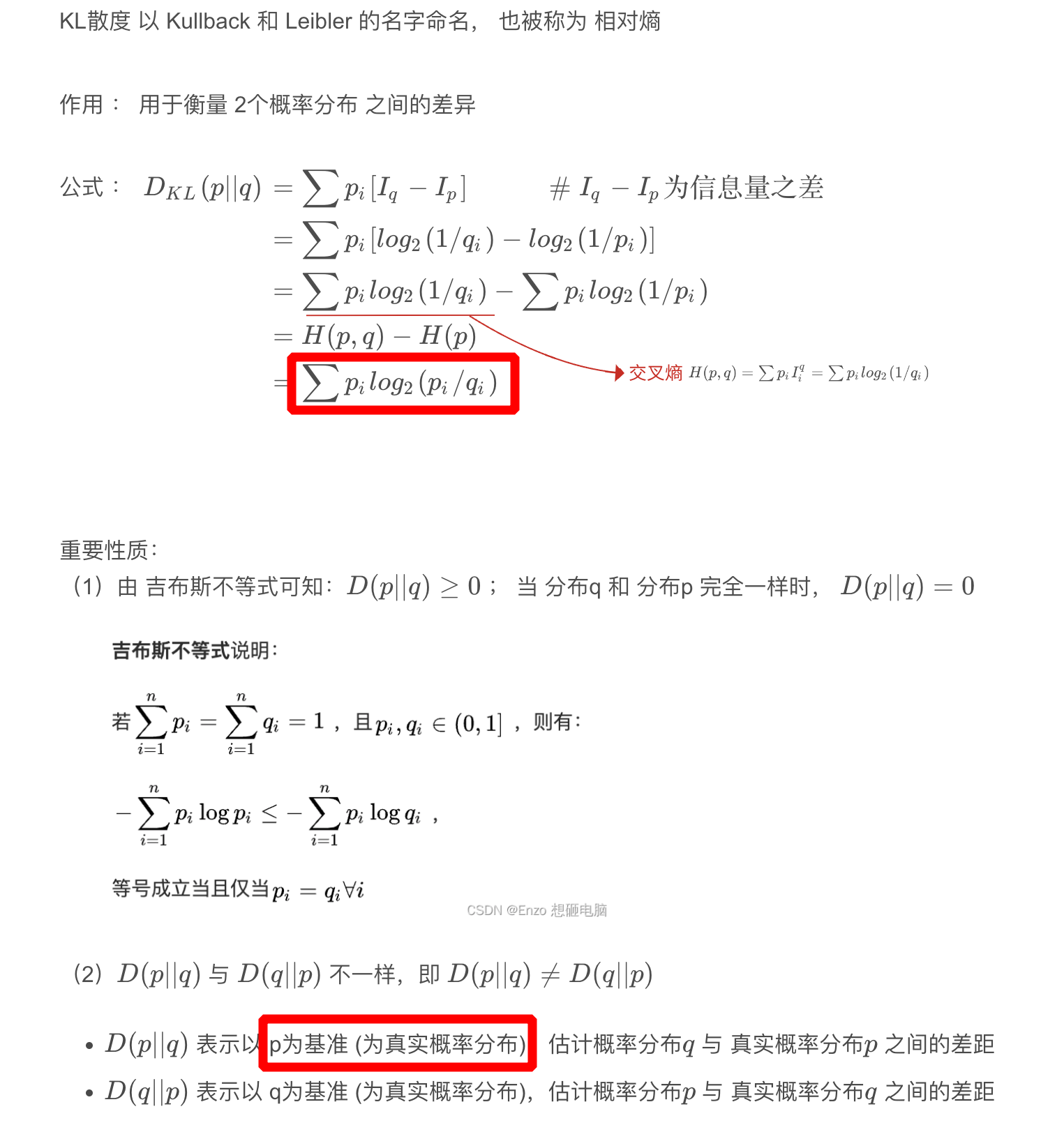
1.3.4、相对熵(KL 散度)
- 相对熵:
- 在熵的基础上,真实概率分布
p保持不变,而信息量换成预测概率分布的信息量与真实概率分布的信息量之差 I q − I p I_q - I_p Iq−Ip - KL 散度用于衡量两个概率分布之间的差异
- 在熵的基础上,真实概率分布
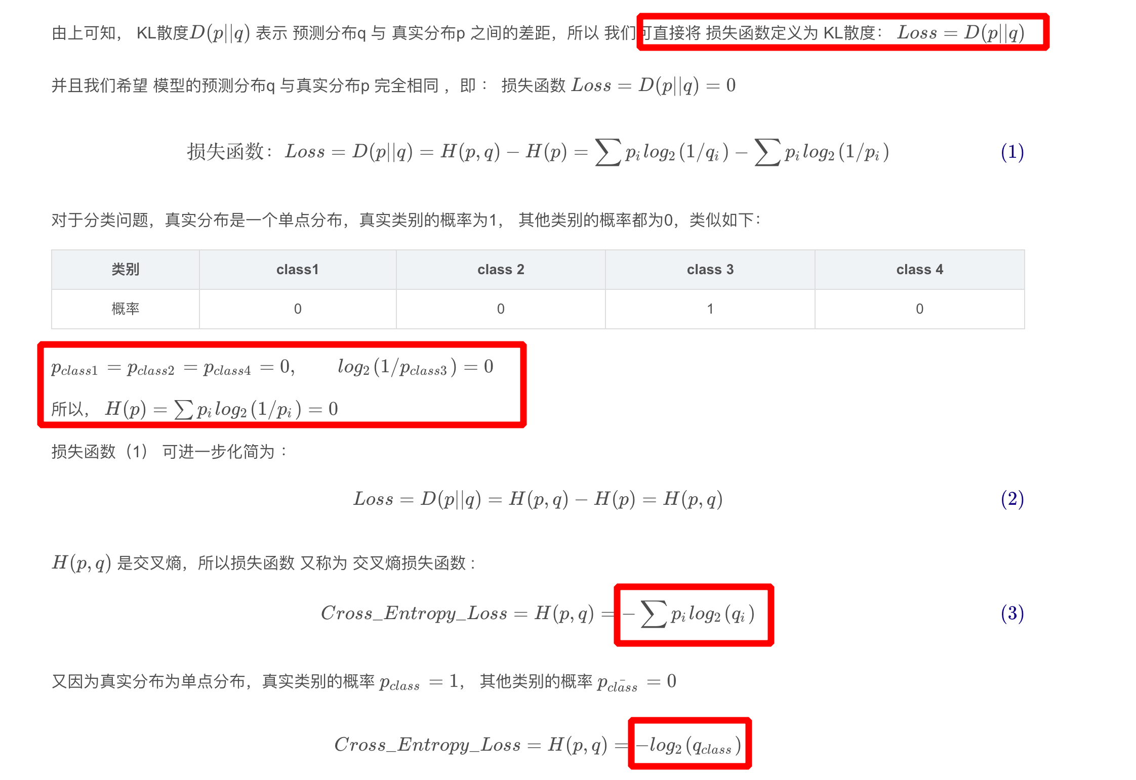
1.3.5、交叉熵损失函数
二、目标检测中的回归损失
1、L1/L2(MSE)/Smooth L1 Loss
- 通过 4 个坐标点独立回归 Building boxes 的缺点:
- 检测
评价方式使用的是 IoU,而实际回归坐标框的时候是使用 4 个坐标点 - 通过4个点回归坐标框的方式是假设 4 个坐标点是相互独立的,没有考虑其
相关性,实际 4 个坐标点具有一定的相关性 - 基于 L1 和 L2 的距离的 loss 对于
尺度不具有不变性(大框较小框损失更大)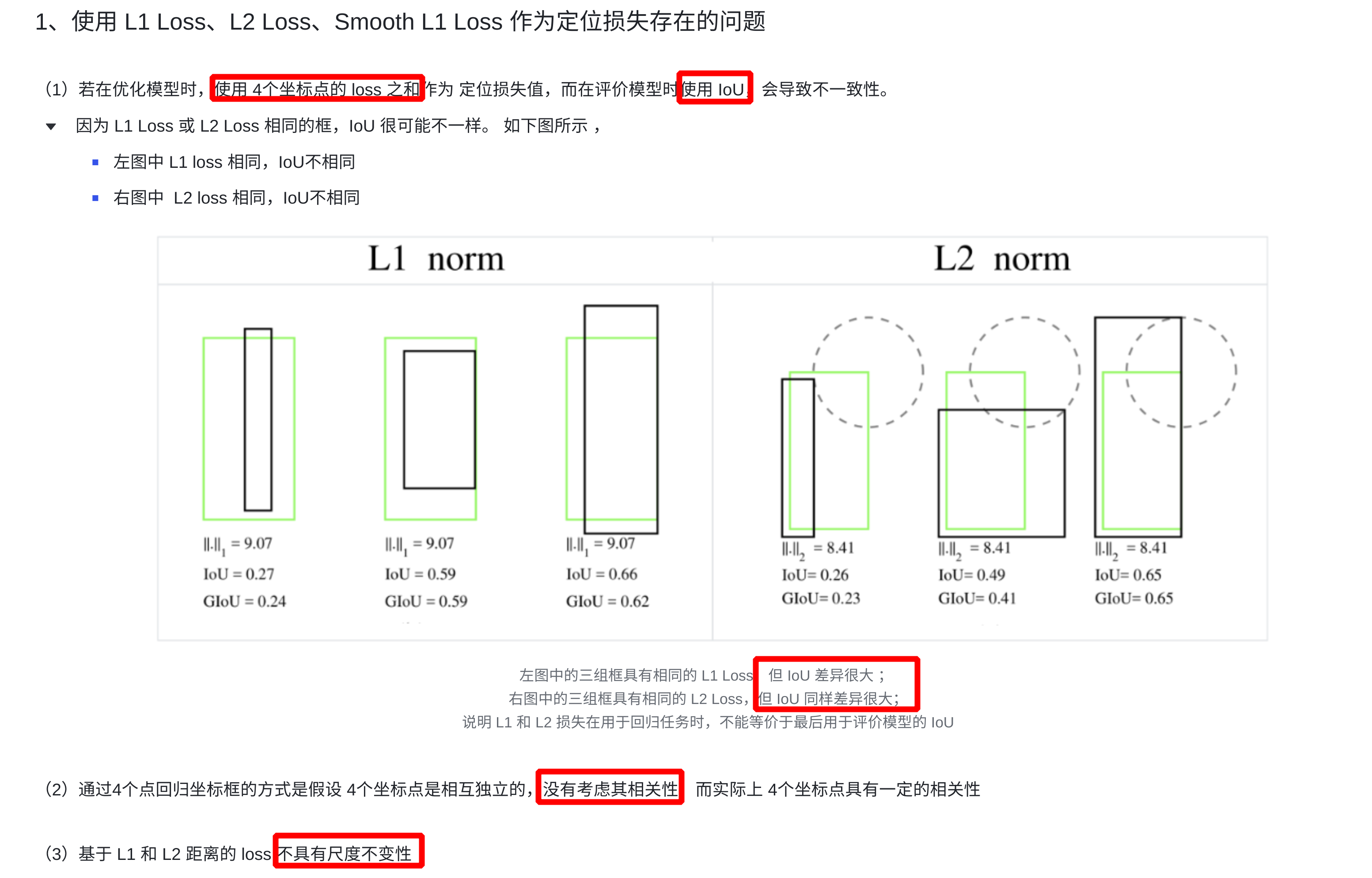
- 检测
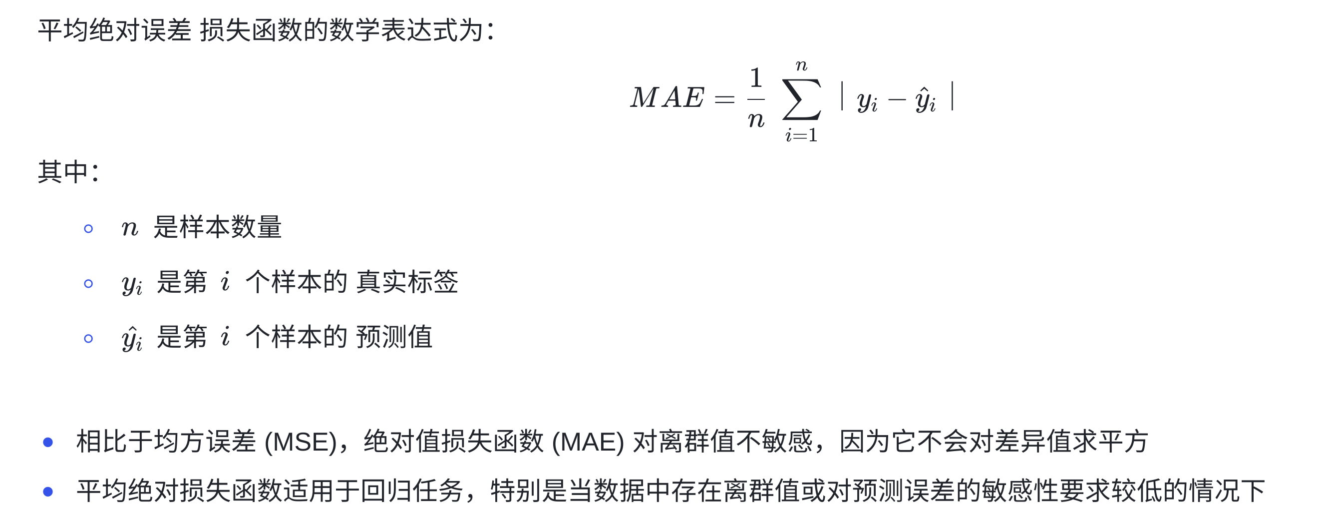
1.1、L1 Loss
- L1 Loss 为平均绝对误差损失函数(MAE :Mean Absolute Error),用于衡量模型对于每个样本预测值与实际值之间的平方差异的平均程度
torch.nn.L1Loss(reduction='mean')  #   参数 reduction :  指定损失的计算方式, 可选值有:"none"、"mean"、"sum"

import torch
import torch.nn as nn

# 创建一个示例输入和目标
torch.manual_seed(121)
predictions = torch.randn((3,))  # 模型的预测值
targets = torch.randn((3,))      # 实际目标值

# 创建 MAE 损失函数实例
mae_loss = nn.L1Loss()

# 计算损失
loss = mae_loss(predictions, targets)

# 打印结果
print('MAE Loss:', loss.item())
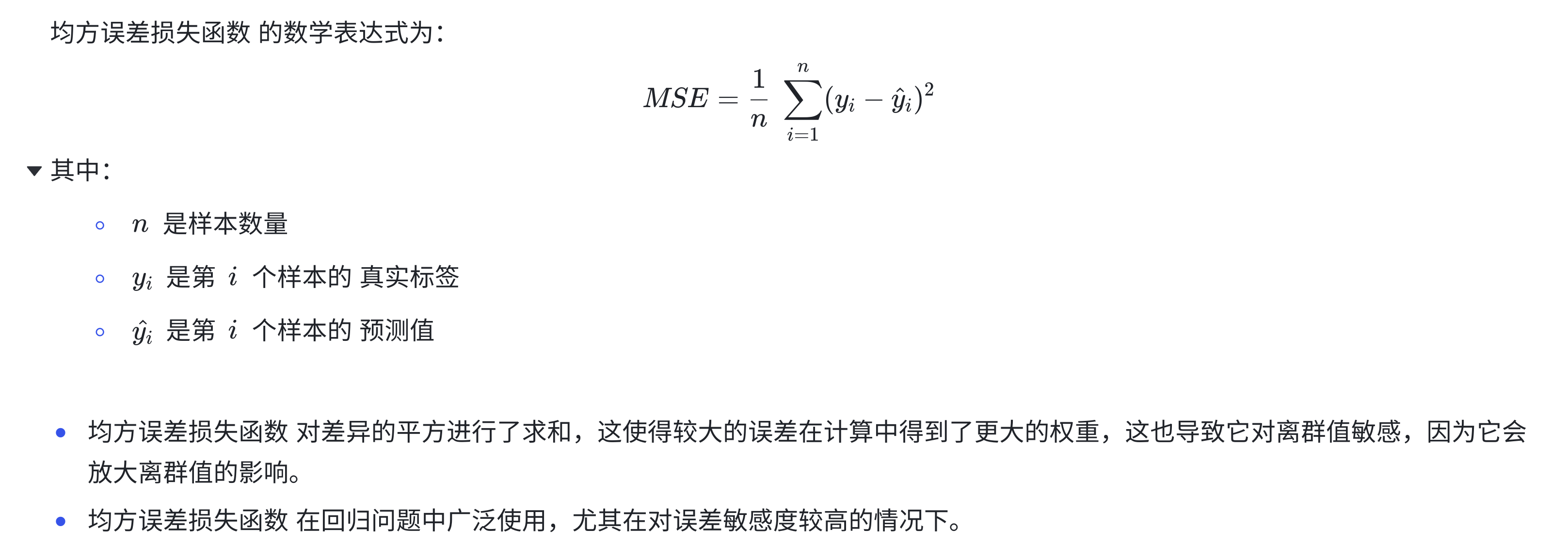
1.2、L2 Loss
- L2 Loss 为均方误差( MSE :Mean Squared Error )损失函数,也称为平方损失函数,用于衡量模型对于每个样本预测值与实际值之间的平方差异的平均程度
torch.nn.MSELoss(reduction='mean')  #   参数 reduction :  指定损失的计算方式, 可选值有:"none"、"mean"、"sum"

import torch
import torch.nn as nn

# 创建一个示例的模型输出和真实标签
torch.manual_seed(121)
model_output = torch.randn(10, requires_grad=True)  # 模型的输出
true_labels = torch.randn(10)  # 真实标签

# 创建均方误差损失函数
mse_loss = nn.MSELoss()

# 计算损失
loss = mse_loss(model_output, true_labels)

# 打印损失值
print("Mean Squared Error Loss:", loss.item())
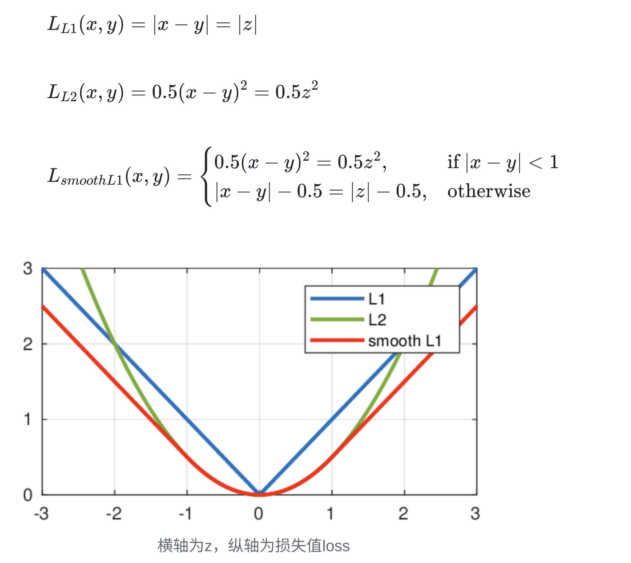
1.3、Smooth L1 Loss
-
Smooth L1 Loss:它对噪声(outliers)更鲁棒,论文中效果较好的参数为 σ = 1.0 \sigma = 1.0 σ=1.0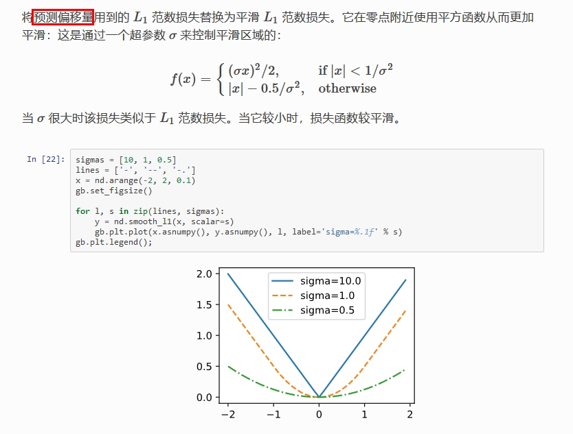
-
Smooth L1 Loss 比 L1 Loss 或 L2 loss 好的原因?
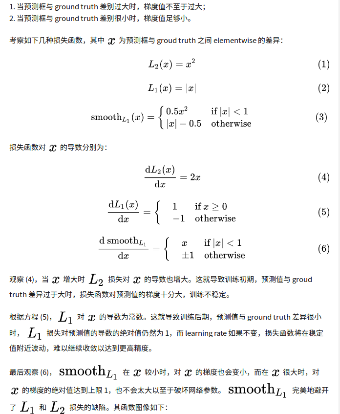
-
代码实现
# smooth-l1-loss
import torch.nn as nn
import torch

loss1 = nn.SmoothL1Loss(reduction='none')
loss2 = nn.SmoothL1Loss(reduction='mean')

torch.manual_seed(121)
y = torch.randn(3)
y_pred = torch.randn(3)

loss_value1 = loss1(y, y_pred)
loss_value2 = loss2(y, y_pred)

print(y)
print(y_pred)
print(loss_value1)
print(loss_value2)


# 手动实现
def smooth_l1_loss(input, target, beta: float = 1. / 9, size_average: bool = True):
    n = torch.abs(input - target)
    cond = torch.lt(n, beta)
    loss = torch.where(cond, 0.5 * n ** 2 / beta, n - 0.5 * beta)
    if size_average:
        return loss.mean()
    return loss.sum()
2、IoU Loss(不用)
-
IoU loss 的优点:解决了 Smooth L1 系列变量
相互独立和不具有尺度不变性(大框较小框损失更大)的两大问题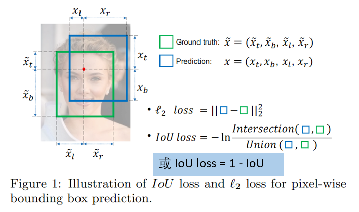
-
IoU loss 的缺点:
- 预测框和真实框不相交时(IOU=0),不能反映出两个框的
距离的远近,此时损失函数不可导,IOU_Loss 无法优化 - 预测框和真实框相交时,无法反映
重合度大小,如下图所示,后面两个具有相同的 IOU,但是 不能反映两个框是如何相交的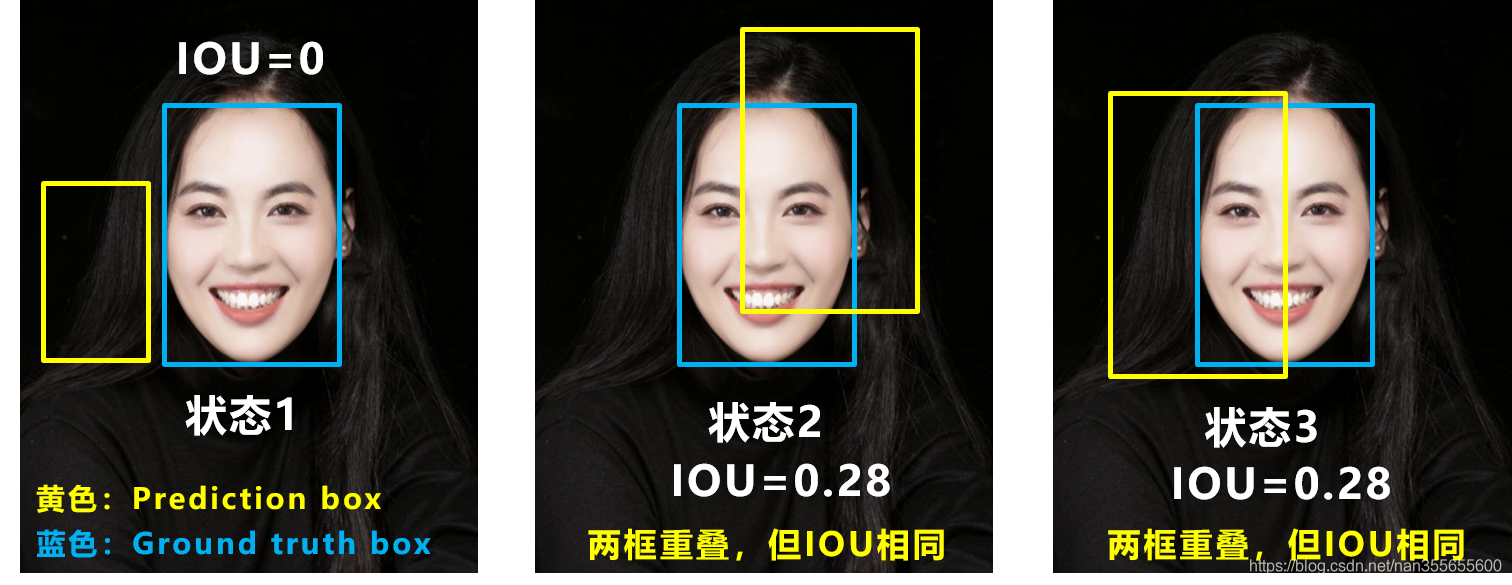
- 预测框和真实框不相交时(IOU=0),不能反映出两个框的
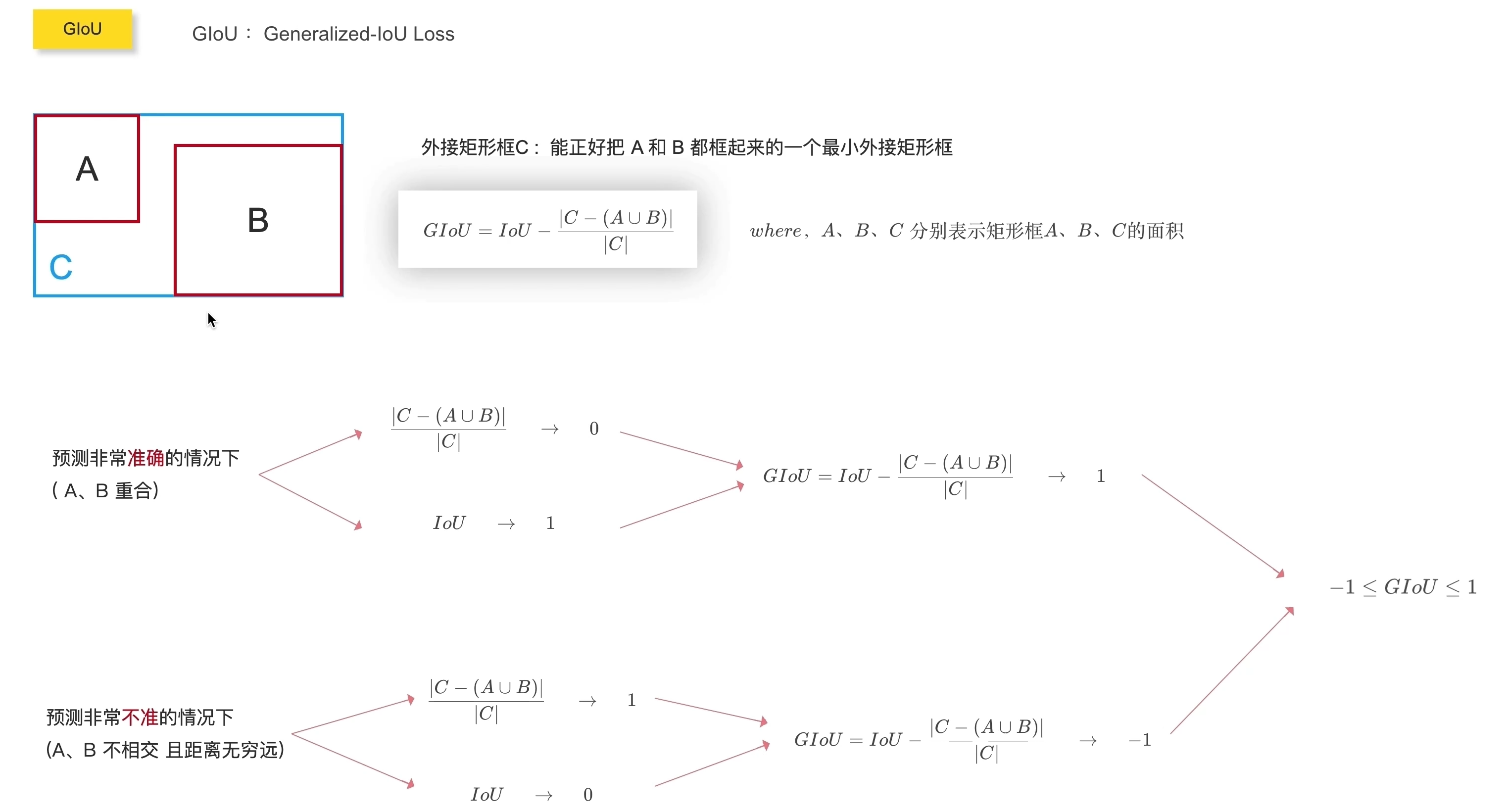
3、GIoU Loss(不用)
- GIoU Loss 的优点:在 IoU 的基础上引入了预测框和真实框的
最小外接矩形- 不仅关注重叠区域,还关注其他的非重叠区域,能更好的反映两者的重合度
- 当预测框和真实框不相交时,由于引入了预测框和真实框的最小外接矩形,最小化 GIoU Loss 会促使 Anchor 和 GT 框不断靠近
- GIoU Loss 的缺点:当两个框属于包含关系时,如下图所示,GIoU 会退化成 IoU,无法区分其相对位置关系(
无法反应中心点距离远近)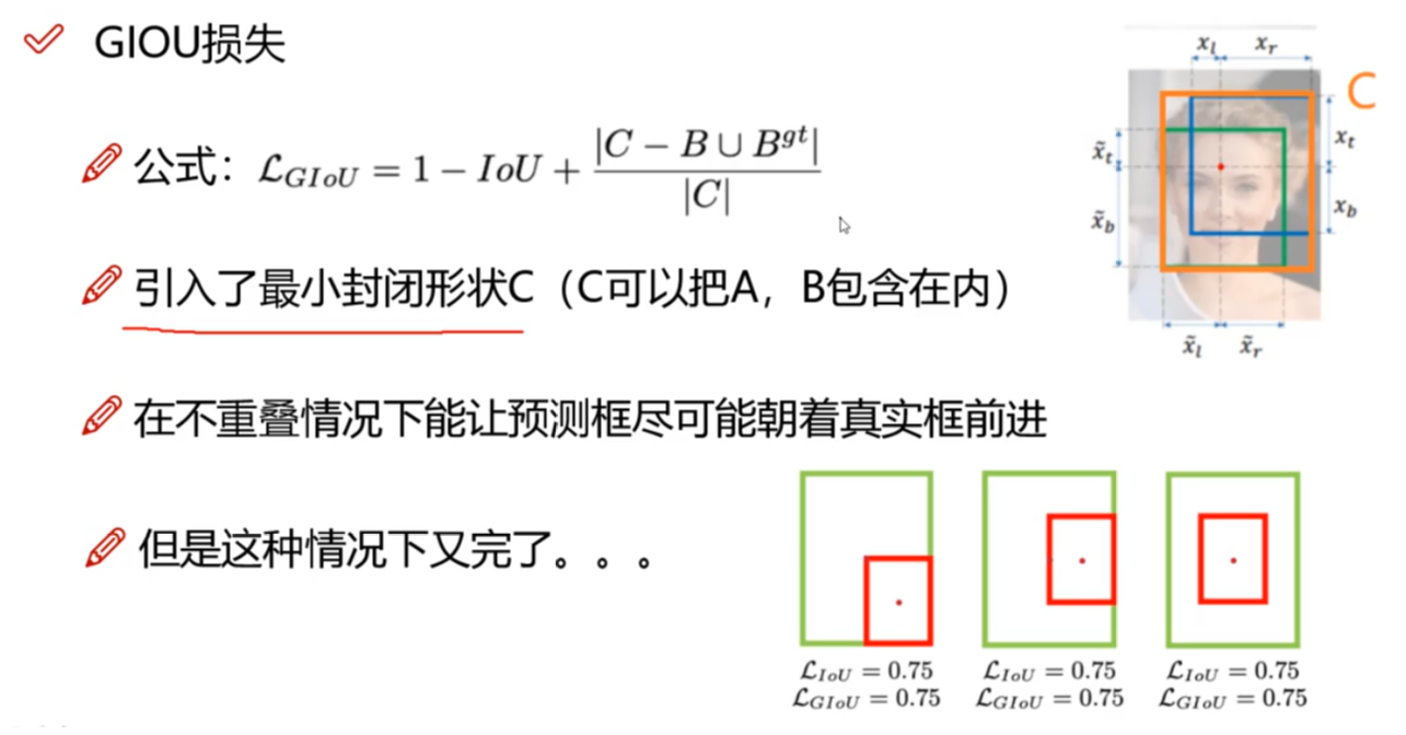
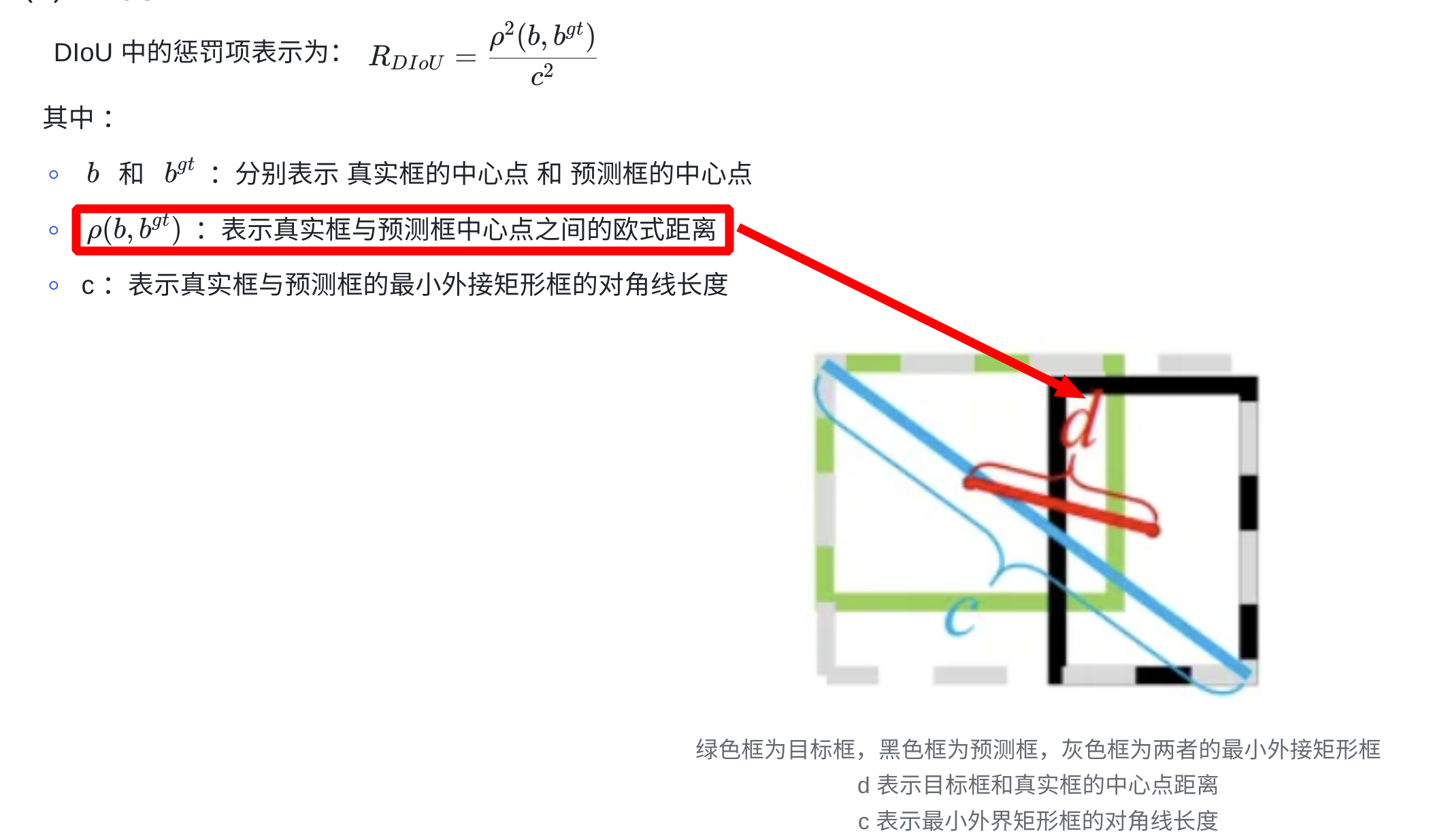
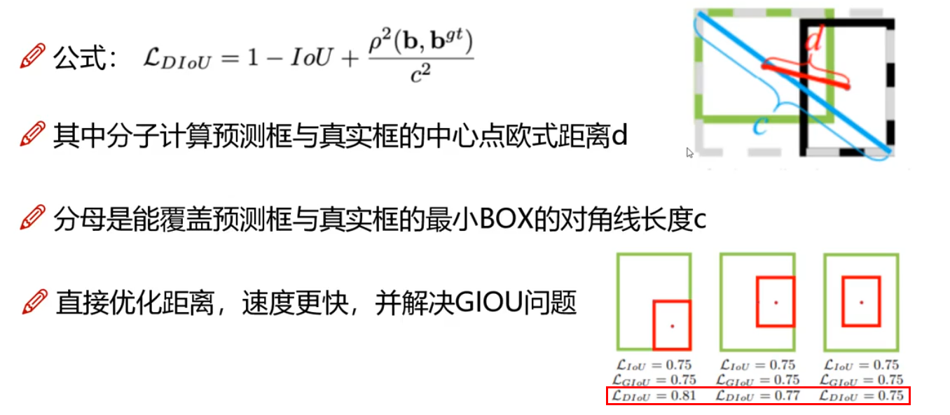
4、DIoU Loss(Distance-IoU Loss–>预测用)
- DIoU 的优点:
- 能够直接最小化预测框和真实框的中心点距离加速收敛
- 还可以替换普通的 IoU 评价策略,应用于NMS 中,使得 NMS 得到的结果更加合理和有效
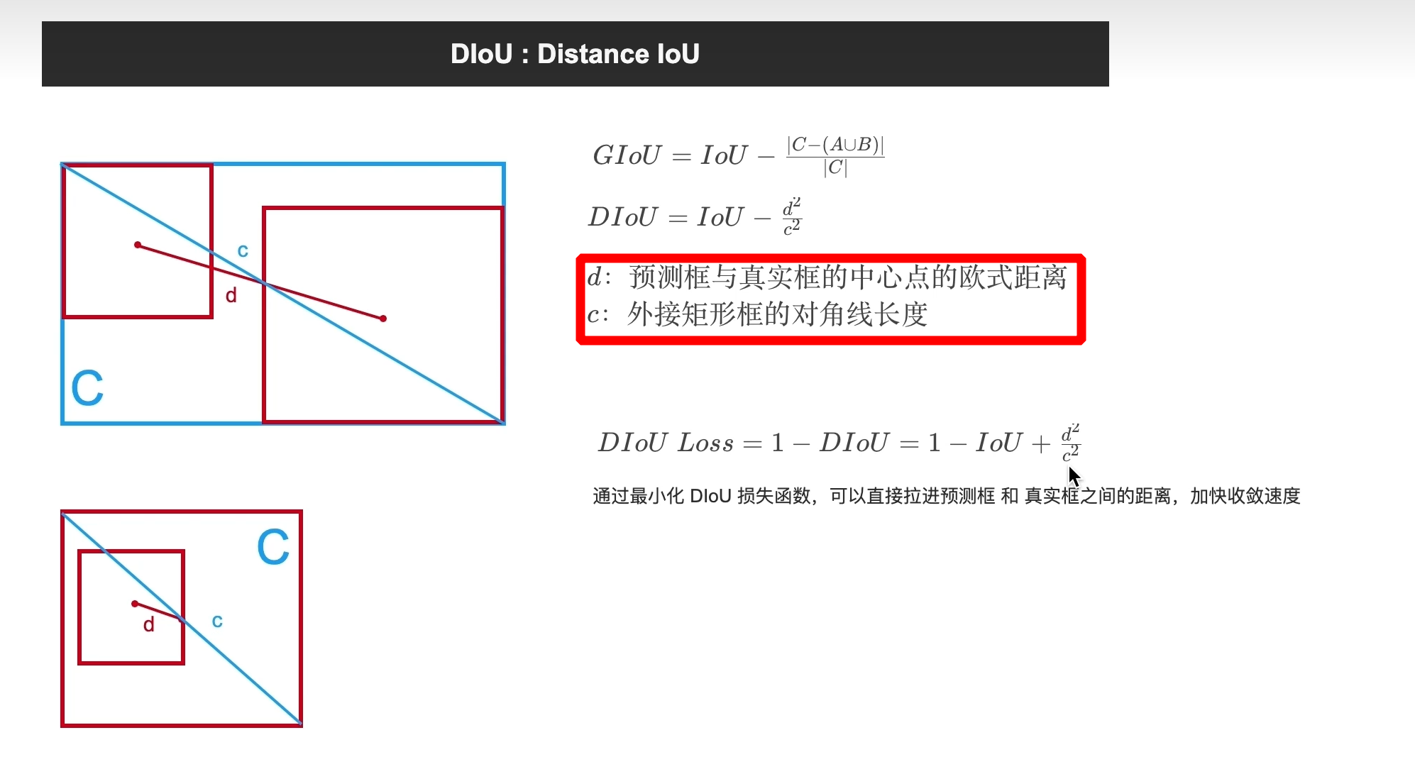
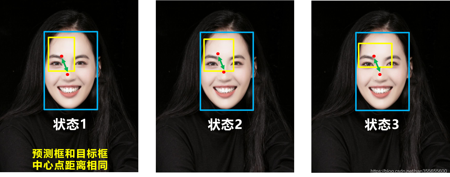
- DIoU 的缺点:未考虑 bbox 回归的长宽比
- 代码实现
import torch


def diou_loss(box1, box2, x1y1x2y2=True):
    '''
    :param box1: 一个 gt bbox, 尺寸为 (4)
    :param box2: 多个 predicted bbox, 尺寸为 (n, 4)
    :param x1y1x2y2: 坐标形式是否为 (xmin, ymin, xmax, ymax)
    :return: 返回 box2 与 bbox1 的 IoU
    '''

    box2 = box2.t()

    if x1y1x2y2:
        b1_x1, b1_y1, b1_x2, b1_y2 = box1[0], box1[1], box1[2], box1[3]
        b2_x1, b2_y1, b2_x2, b2_y2 = box2[0], box2[1], box2[2], box2[3]
    else:  # 将坐标形式由 (cx, cy, w, h) 转换为 (xmin, ymin, xmax, ymax)
        b1_x1, b1_x2 = box1[0] - box1[2] / 2, box1[0] + box1[2] / 2
        b1_y1, b1_y2 = box1[1] - box1[3] / 2, box1[1] + box1[3] / 2
        b2_x1, b2_x2 = box2[0] - box2[2] / 2, box2[0] + box2[2] / 2
        b2_y1, b2_y2 = box2[1] - box2[3] / 2, box2[1] + box2[3] / 2

    # Intersection area
    inter = (torch.min(b1_x2, b2_x2) - torch.max(b1_x1, b2_x1)).clamp(0) * \
            (torch.min(b1_y2, b2_y2) - torch.max(b1_y1, b2_y1)).clamp(0)

    # Union Area
    w1, h1 = b1_x2 - b1_x1, b1_y2 - b1_y1
    w2, h2 = b2_x2 - b2_x1, b2_y2 - b2_y1
    union = w1 * h1 + w2 * h2 - inter + 1e-16

    # iou
    iou = inter / union

    # external rectangle box
    cw = torch.max(b1_x2, b2_x2) - torch.min(b1_x1, b2_x1)
    ch = torch.max(b1_y2, b2_y2) - torch.min(b1_y1, b2_y1)

    # external rectangle box area squared
    c2 = cw ** 2 + ch ** 2 + 1e-16

    # centerpoint distance squared
    rho2 = ((b2_x1 + b2_x2) - (b1_x1 + b1_x2)) ** 2 / 4 + ((b2_y1 + b2_y2) - (b1_y1 + b1_y2)) ** 2 / 4

    return 1 - iou + rho2 / c2


if __name__ == '__main__':
    box1 = torch.tensor([1.0, 2.0, 5.0, 6.0])  # 一个gt bbox的坐标
    box2 = torch.tensor([[1.0, 2.0, 4.0, 5.0], [3.0, 4.0, 7.0, 8.0]])  # 2个预测的bbox的坐标

    loss = diou_loss(box1, box2)
    print(loss)
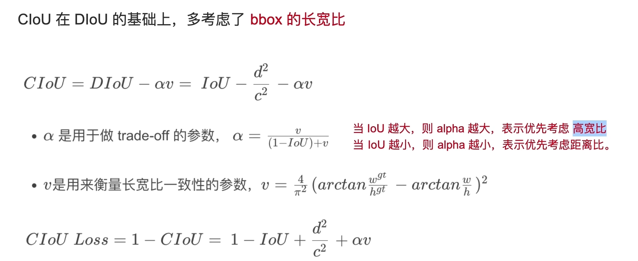
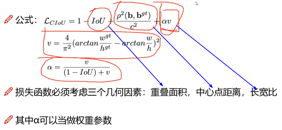
5、CIoU Loss(Complete-IoU Loss–>训练用)
-
α \alpha α 是权重平衡因子,调整长宽比的影响
-
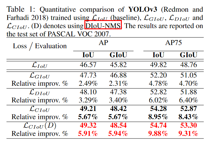
CIoU 优点:在 DIoU 的基础上将 bbox 的长宽比考虑到损失函数中,进一步提升了回归精度
-
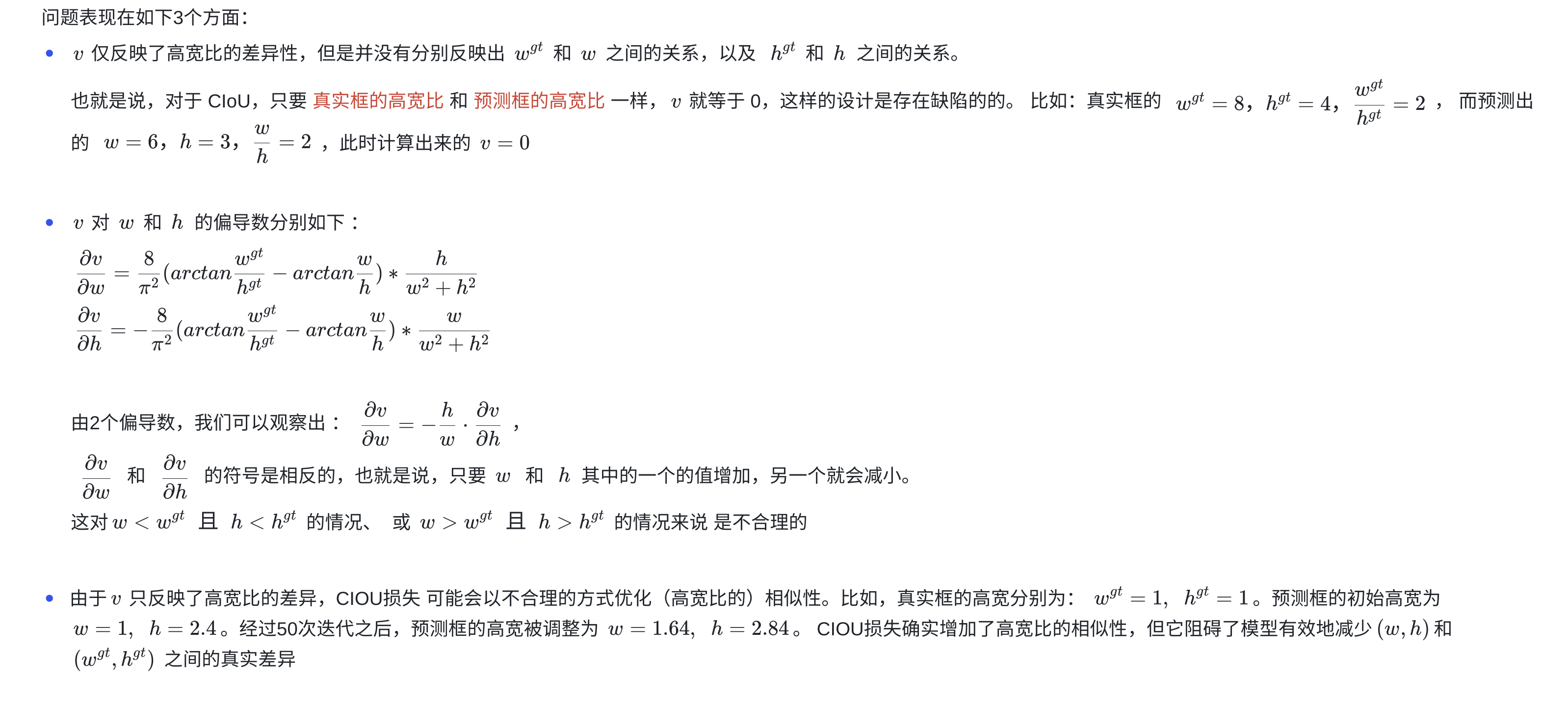
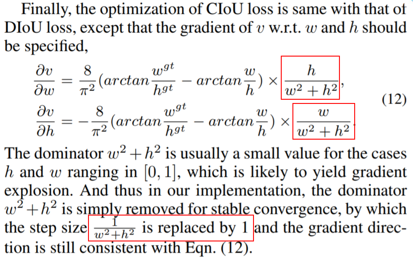
CIoU 缺点: α v \alpha v αv 这一项的设计还是存在问题,导致拖累了收敛速度
-
求导注意事项:
-
代码实现
import torch
import math


def ciou_loss(box1, box2, x1y1x2y2=True):
    '''
    :param box1: 一个 gt bbox, 尺寸为 (4)
    :param box2: 多个 predicted bbox, 尺寸为 (n, 4)
    :param x1y1x2y2: 坐标形式是否为 (xmin, ymin, xmax, ymax)
    :return: 返回 box2 与 bbox1 的 IoU
    '''

    box2 = box2.t()

    if x1y1x2y2:
        b1_x1, b1_y1, b1_x2, b1_y2 = box1[0], box1[1], box1[2], box1[3]
        b2_x1, b2_y1, b2_x2, b2_y2 = box2[0], box2[1], box2[2], box2[3]
    else:  # 将坐标形式由 (cx, cy, w, h) 转换为 (xmin, ymin, xmax, ymax)
        b1_x1, b1_x2 = box1[0] - box1[2] / 2, box1[0] + box1[2] / 2
        b1_y1, b1_y2 = box1[1] - box1[3] / 2, box1[1] + box1[3] / 2
        b2_x1, b2_x2 = box2[0] - box2[2] / 2, box2[0] + box2[2] / 2
        b2_y1, b2_y2 = box2[1] - box2[3] / 2, box2[1] + box2[3] / 2

    # Intersection area
    inter = (torch.min(b1_x2, b2_x2) - torch.max(b1_x1, b2_x1)).clamp(0) * \
            (torch.min(b1_y2, b2_y2) - torch.max(b1_y1, b2_y1)).clamp(0)

    # Union Area
    w1, h1 = b1_x2 - b1_x1, b1_y2 - b1_y1
    w2, h2 = b2_x2 - b2_x1, b2_y2 - b2_y1
    union = w1 * h1 + w2 * h2 - inter + 1e-16

    # iou
    iou = inter / union

    # external rectangle box
    cw = torch.max(b1_x2, b2_x2) - torch.min(b1_x1, b2_x1)
    ch = torch.max(b1_y2, b2_y2) - torch.min(b1_y1, b2_y1)

    # external rectangle box area squared
    c2 = cw ** 2 + ch ** 2 + 1e-16

    # centerpoint distance squared
    rho2 = ((b2_x1 + b2_x2) - (b1_x1 + b1_x2)) ** 2 / 4 + ((b2_y1 + b2_y2) - (b1_y1 + b1_y2)) ** 2 / 4

    v = (4 / math.pi ** 2) * torch.pow(torch.atan(w2 / h2) - torch.atan(w1 / h1), 2)
    with torch.no_grad():
        alpha = v / (1 - iou + v)
    return 1 - iou + (rho2 / c2 + v * alpha)


if __name__ == '__main__':

    box1 = torch.tensor([1.0, 2.0, 5.0, 6.0])  # 一个gt bbox的坐标
    box2 = torch.tensor([[1.0, 2.0, 4.0, 5.0], [3.0, 4.0, 7.0, 8.0]])  # 2个预测的bbox的坐标

    loss = ciou_loss(box1, box2)
    print(loss)
6、各种 IoU based loss 的效果及代码实现
- 最近几年还有 EIoU、SIoU、Shape IoU 等新方法出现
def bbox_iou(box1, box2, x1y1x2y2=True, GIoU=False, DIoU=False, CIoU=False, eps=1e-7):
    # Returns the IoU of box1 to box2. box1 is 4, box2 is nx4
    box2 = box2.T

    # Get the coordinates of bounding boxes
    if x1y1x2y2:  # x1, y1, x2, y2 = box1
        b1_x1, b1_y1, b1_x2, b1_y2 = box1[0], box1[1], box1[2], box1[3]
        b2_x1, b2_y1, b2_x2, b2_y2 = box2[0], box2[1], box2[2], box2[3]
    else:  # transform from xywh to xyxy
        b1_x1, b1_x2 = box1[0] - box1[2] / 2, box1[0] + box1[2] / 2
        b1_y1, b1_y2 = box1[1] - box1[3] / 2, box1[1] + box1[3] / 2
        b2_x1, b2_x2 = box2[0] - box2[2] / 2, box2[0] + box2[2] / 2
        b2_y1, b2_y2 = box2[1] - box2[3] / 2, box2[1] + box2[3] / 2

    # Intersection area
    inter = (torch.min(b1_x2, b2_x2) - torch.max(b1_x1, b2_x1)).clamp(0) * \
            (torch.min(b1_y2, b2_y2) - torch.max(b1_y1, b2_y1)).clamp(0)

    # Union Area
    w1, h1 = b1_x2 - b1_x1, b1_y2 - b1_y1 + eps
    w2, h2 = b2_x2 - b2_x1, b2_y2 - b2_y1 + eps
    union = w1 * h1 + w2 * h2 - inter + eps

    iou = inter / union
    if GIoU or DIoU or CIoU:
    	# 计算闭包区域
        cw = torch.max(b1_x2, b2_x2) - torch.min(b1_x1, b2_x1)  # convex (smallest enclosing box) width
        ch = torch.max(b1_y2, b2_y2) - torch.min(b1_y1, b2_y1)  # convex height
        if CIoU or DIoU:  # Distance or Complete IoU https://arxiv.org/abs/1911.08287v1
            c2 = cw ** 2 + ch ** 2 + eps  # convex diagonal squared
            rho2 = ((b2_x1 + b2_x2 - b1_x1 - b1_x2) ** 2 +
                    (b2_y1 + b2_y2 - b1_y1 - b1_y2) ** 2) / 4  # center distance squared,计算中心点距离
            if DIoU:
                return iou - rho2 / c2  # DIoU
            elif CIoU:  # https://github.com/Zzh-tju/DIoU-SSD-pytorch/blob/master/utils/box/box_utils.py#L47
                v = (4 / math.pi ** 2) * torch.pow(torch.atan(w2 / h2) - torch.atan(w1 / h1), 2)
                with torch.no_grad():
                    alpha = v / (v - iou + (1 + eps))
                return iou - (rho2 / c2 + v * alpha)  # CIoU
        else:  # GIoU https://arxiv.org/pdf/1902.09630.pdf
            c_area = cw * ch + eps  # convex area
            return iou - (c_area - union) / c_area  # GIoU
    else:
        return iou  # IoU
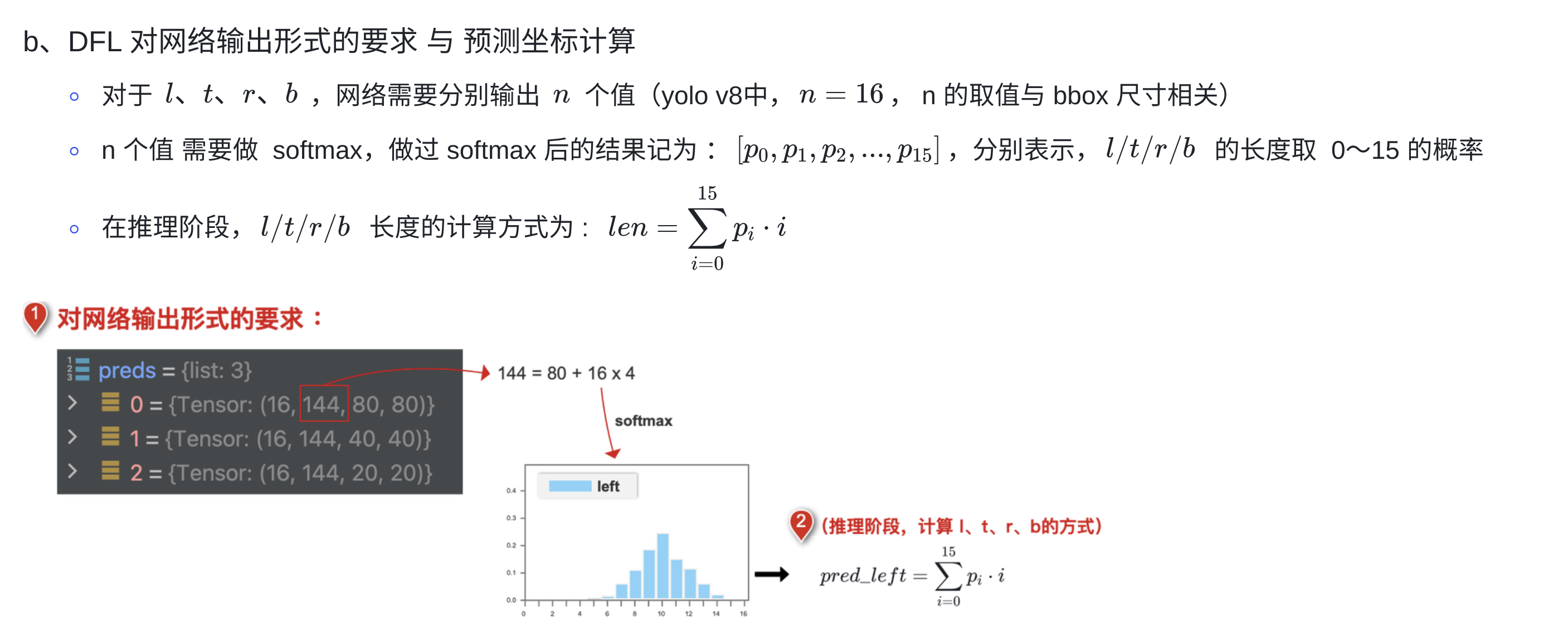
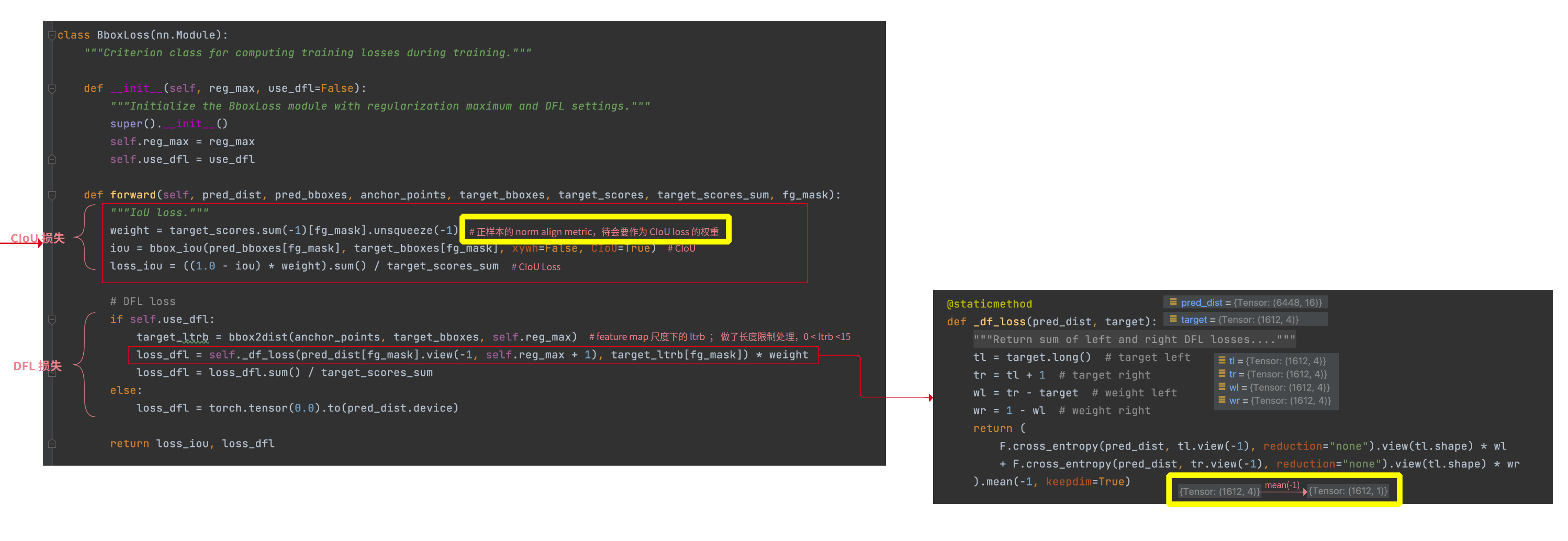
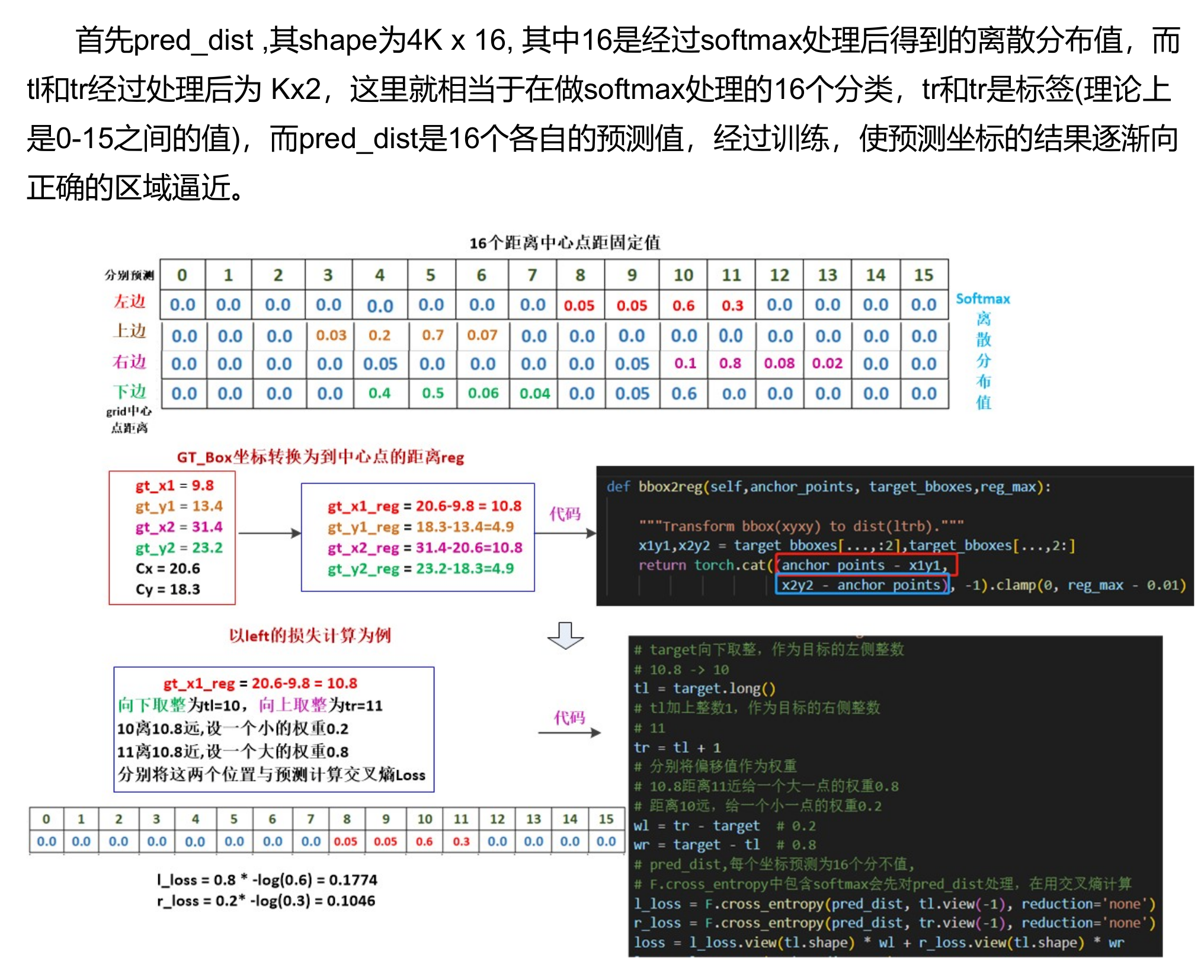
7、DFL Loss
-
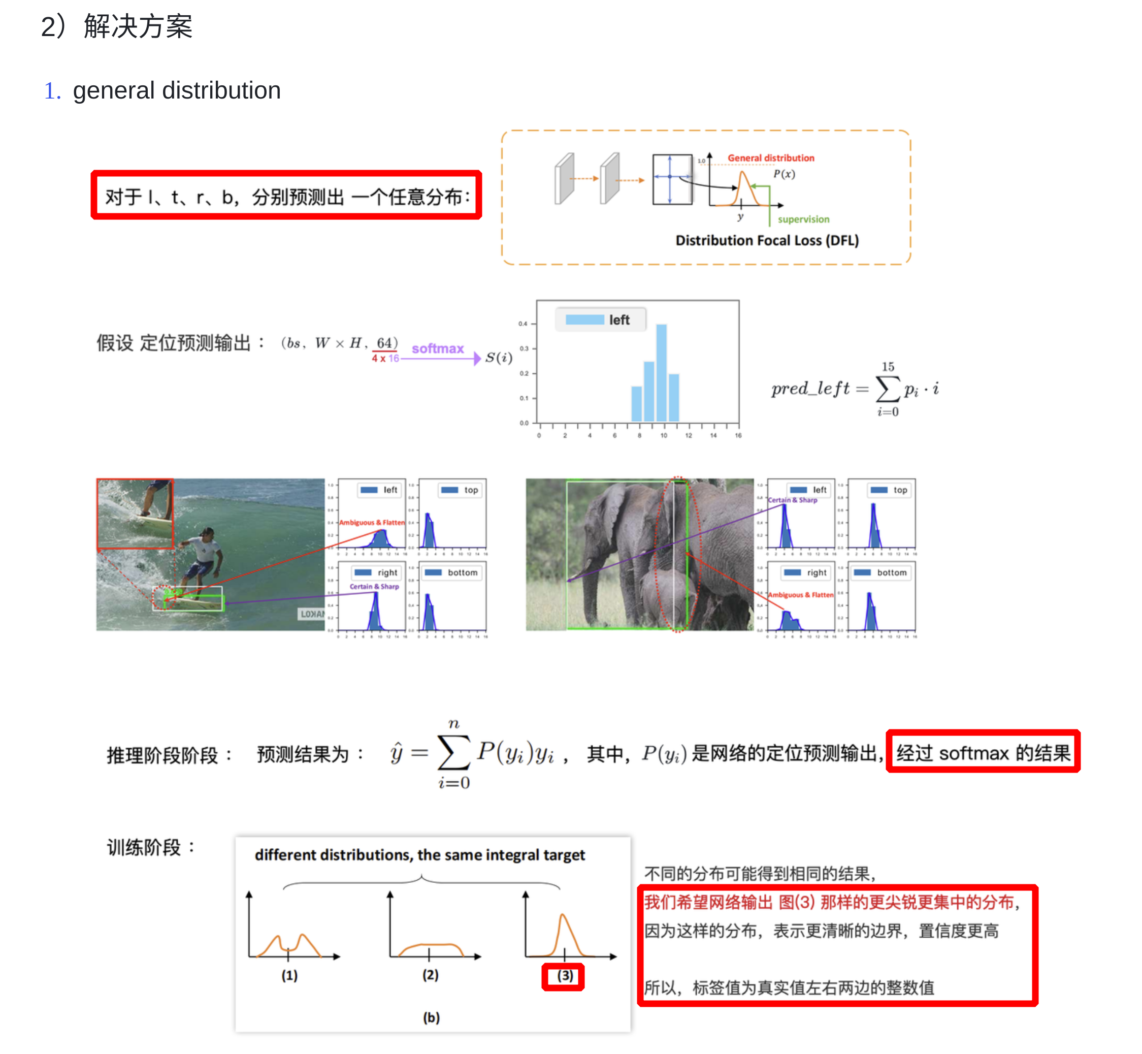
bbox 坐标的预测结果,服从狄拉克分布,对于
l、t、r、b网络分布只预测出一个值,预测出的值的概率为 1,其它值的概率都为 0 -
DFL:将框的位置建模成一个
general distribution,让网络快速的聚焦于和目标位置距离近的位置的分布;对于l、t、r、b会让网络分布输出多个值,这些值服从任意分布,每个值有自己对应的概率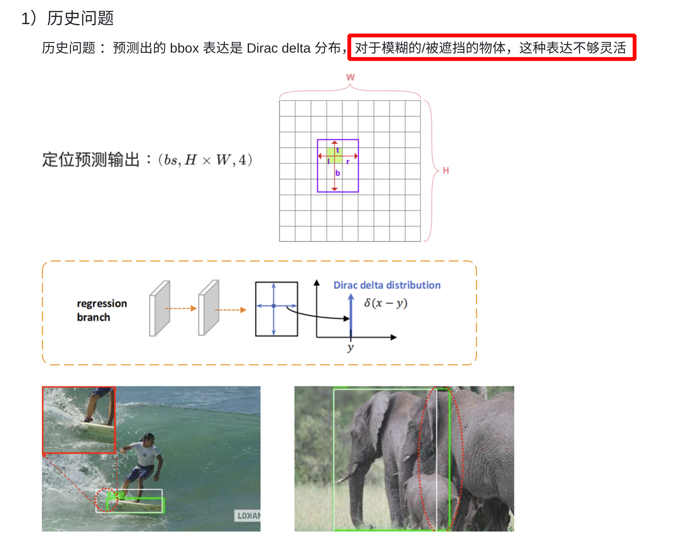
-
推理阶段
-
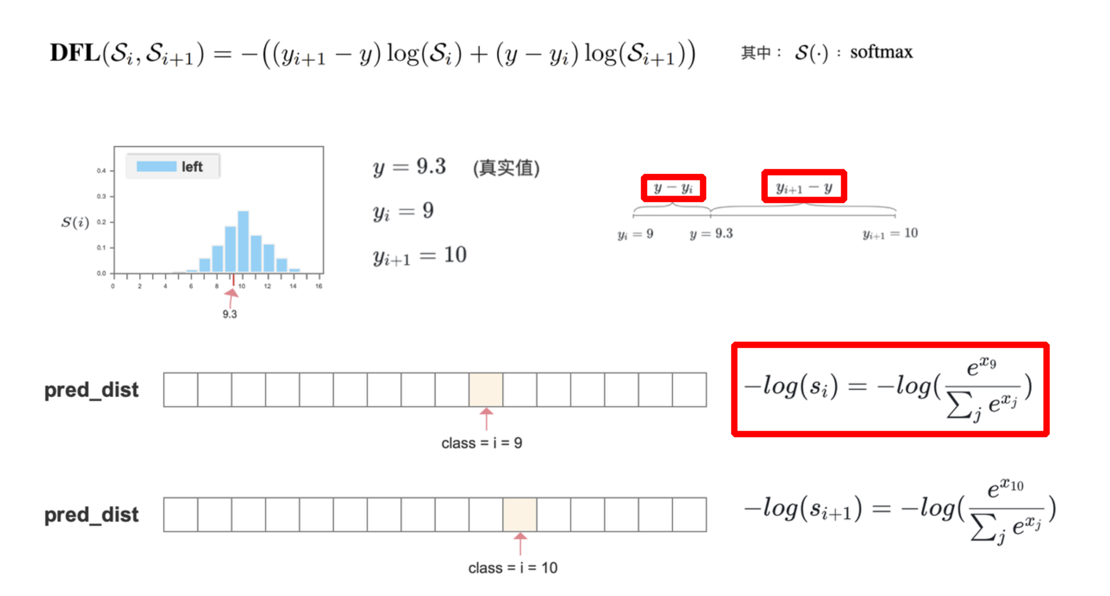
训练阶段:
- 真实值坐标左边的值(
y-向下取整)和右边的值(向上取整-y)作为真实标签 - 以
交叉熵的形式去优化与标签 y 最接近的一左一右2个位置的概率,从而让网络更快地聚焦到目标位置的邻近区域的分布;也就是说学出来的分布,理论上是在真实浮点坐标的附近,并且以线性插值的模式得到距离左右整数坐标的权重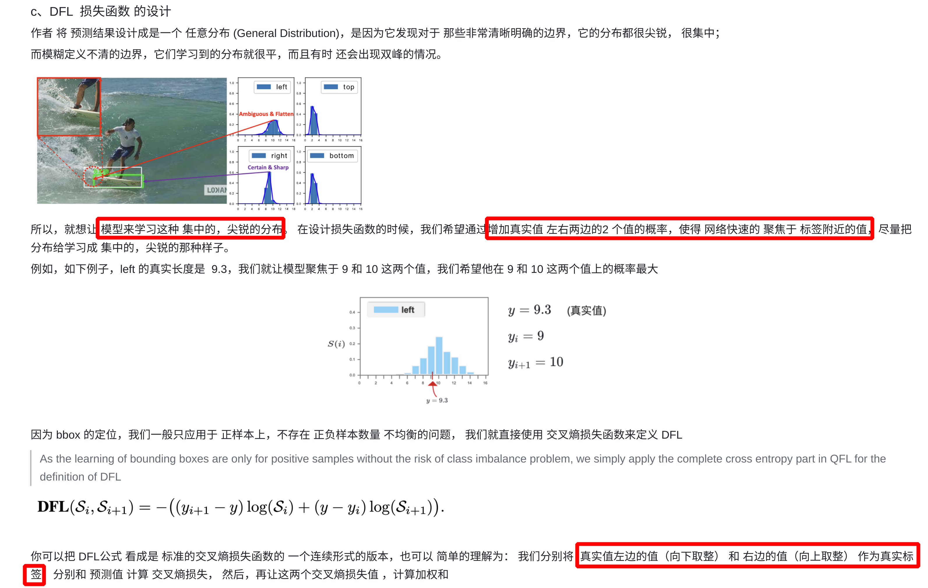
- 真实值坐标左边的值(
- 代码实现
# https://github.com/ultralytics/ultralytics/blob/62180db48cf8e5b6a3946b3f63f109d81e14ad0f/ultralytics/utils/loss.py#L78
class DFLoss(nn.Module):
    """Criterion class for computing Distribution Focal Loss (DFL)."""

    def __init__(self, reg_max=16) -> None:
        """Initialize the DFL module with regularization maximum."""
        super().__init__()
        self.reg_max = reg_max

    def __call__(self, pred_dist, target):
        """Return sum of left and right DFL losses from https://ieeexplore.ieee.org/document/9792391."""
        target = target.clamp_(0, self.reg_max - 1 - 0.01)
        tl = target.long()  # target left
        tr = tl + 1  # target right
        wl = tr - target  # weight left
        wr = 1 - wl  # weight right
        return (
            F.cross_entropy(pred_dist, tl.view(-1), reduction="none").view(tl.shape) * wl
            + F.cross_entropy(pred_dist, tr.view(-1), reduction="none").view(tl.shape) * wr
        ).mean(-1, keepdim=True)
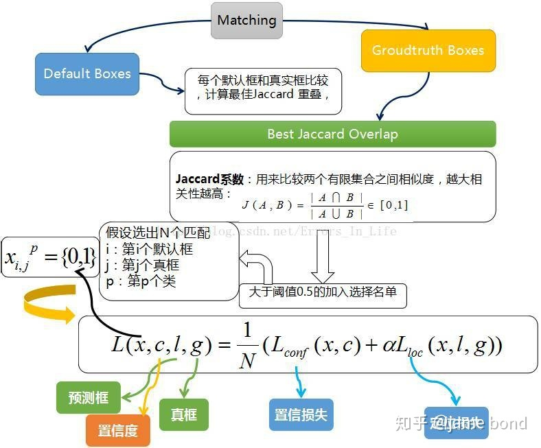
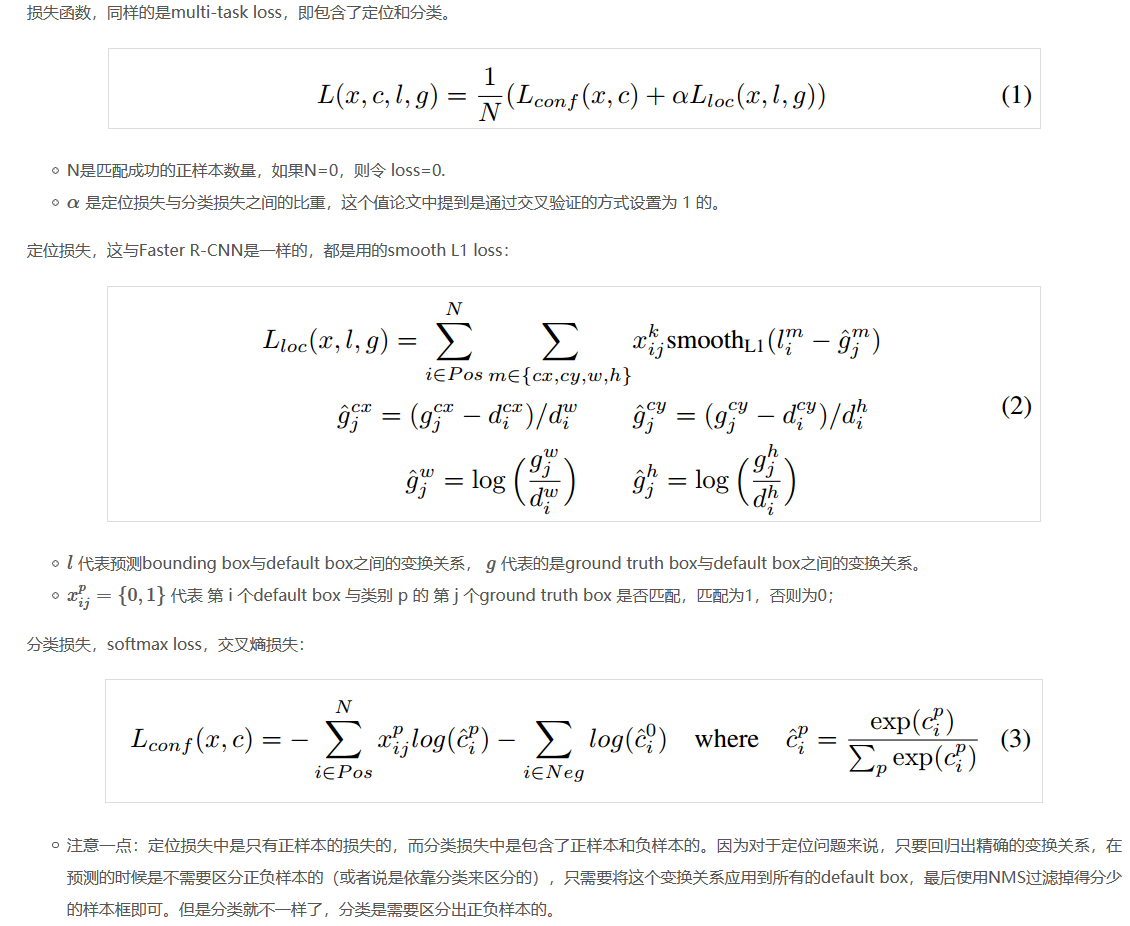
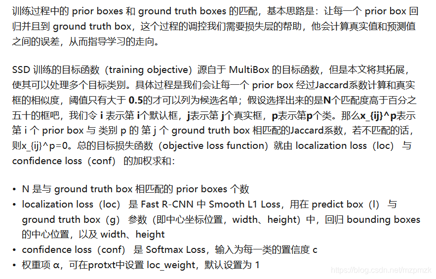
三、SSD 中的损失函数
四、目标检测中回归的原理
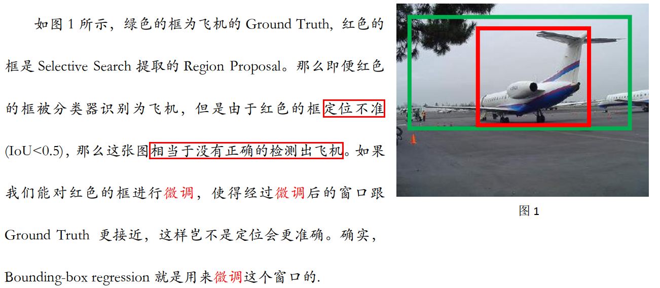
1、为什么要做 bbox regression?
回归目的:提高目标定位的精度!
2、回归的对象是什么?
回归对象:相对 prior box(anchor box or propoal) 的平移和缩放量,这样可以使得模型有一个较好的搜索起点
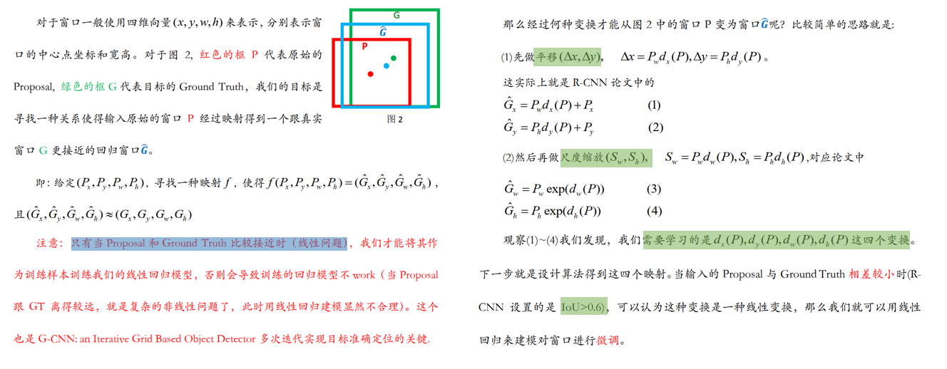
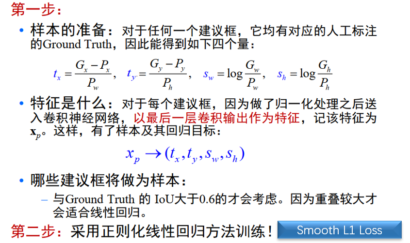
3、回归模型怎么训练?
- 训练方法:
- 对每一个 prior box(anchor box or propoal) 进行 labeling,只选取其中的正样本(eg: IoU>0.6)来做回归
- 计算 prior box 和其对应的 groud truth box 间的平移和缩放量
- 注意:这里的平移和缩放量
除以了prior box 的宽和高(宽和高变换到对数域)做归一化处理,因为图像中各个框的位置远近以及形状大小各异,这样做能使偏移量的分布更均匀从而更容易拟合
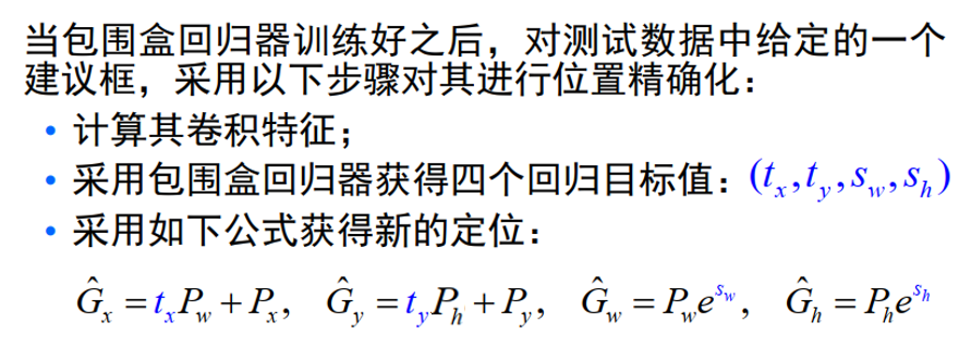
4、回归模型怎么测试?
输入:prior box 的坐标 ( P x , P y , P w , P h ) (P_x, P_y, P_w, P_h) (Px,Py,Pw,Ph),其实真正的输入是这个窗口对应的
CNN 特征
输出:prior box 经过模型回归后的坐标 ( t x , t y , s w , s h ) (t_x, t_y, s_w, s_h) (tx,ty,sw,sh),然后再做一下反归一化就可以得到其真实坐标
// 注意这里加了 prior_variance 参数(便于梯度更好的回传),一般为 [0.1, 0.1, 0.2, 0.2]
// variance is encoded in bbox, we need to scale the offset accordingly.
decode_bbox_center_x = prior_variance[0] * bbox.xmin() * prior_width + prior_center_x;
decode_bbox_center_y = prior_variance[1] * bbox.ymin() * prior_height + prior_center_y;
decode_bbox_width = exp(prior_variance[2] * bbox.xmax()) * prior_width;
decode_bbox_height = exp(prior_variance[3] * bbox.ymax()) * prior_height;

// 然后转成两个坐标的形式
decode_bbox->set_xmin(decode_bbox_center_x - decode_bbox_width / 2.);
decode_bbox->set_ymin(decode_bbox_center_y - decode_bbox_height / 2.);
decode_bbox->set_xmax(decode_bbox_center_x + decode_bbox_width / 2.);
decode_bbox->set_ymax(decode_bbox_center_y + decode_bbox_height / 2.);
五、参考资料
1、TensorFLow 中的损失函数
2、请问faster rcnn和ssd 中为什么用smooth l1 loss,和l2有什么区别?
3、L1&L2 正则化
4、bounding box regression detail(CaffeCN)
5、论文阅读: RetinaNet !!
6、何恺明大神的「Focal Loss」,如何更好地理解?
7、5分钟理解Focal Loss与GHM——解决样本不平衡利器 !!!
8、Imbalance Problems in Object Detection: A Review
9、详解各种iou损失函数的计算方式(iou、giou、ciou、diou)

有“AI”的1024 = 2048,欢迎大家加入2048 AI社区
更多推荐


 0
0 0
0- 0


 已为社区贡献18条内容

所有评论(0)