注意：本文引用自专业人工智能社区Venus AI

更多AI知识请参考原站 （[www.aideeplearning.cn]）

项目背景

客户个性分析是对公司理想客户的详细分析，有助于企业更好地了解其客户，以满足不同类型客户的特定需求、行为和关注点。通过客户个性分析，企业可以更精确地调整其产品、服务和市场策略，提高客户满意度和业务绩效。

项目目标

本项目的主要目标是进行客户个性分析，通过聚类客户，识别不同类型的客户群体。我们的目标是回答以下问题：

1. 人们对产品的评价：是什么决定了客户对产品的态度。
2. 人们做了什么：揭示了人们在做什么，而不是他们对产品的评价。

项目应用

客户个性分析在市场营销和业务决策中具有广泛的应用。一些潜在的应用包括：

• 定制市场策略：根据不同客户群体的需求和偏好，调整产品推广和定价策略。
• 提高客户满意度：根据客户个性，提供更个性化的客户支持和服务。
• 产品优化：根据客户反馈和行为，改进产品设计和功能。

数据集

我们使用的数据集包含了客户的各种属性，包括出生年份、教育程度、婚姻状况、家庭年收入、家庭成员数量、投诉历史、购买历史等。这些属性将帮助我们了解客户的特点和行为。

属性

• ID：客户的唯一标识符
• Year_Birth：客户的出生年份
• Education：客户的教育程度
• Marital_Status：客户的婚姻状况
• Income：客户的家庭年收入
• Kidhome：客户家庭中的儿童数量
• Teenhome：客户家庭中青少年的数量
• Dt_Customer：客户在公司注册的日期
• Recency：自客户上次购买以来的天数
• Complain：如果客户在过去 2 年内投诉过，则为 1，否则为 0 产品

---

• MntWines：过去 2 年在葡萄酒上的花费金额
• MntFruits：过去 2 年在水果上花费的金额
• MntMeatProducts：过去 2 年在肉类上的花费金额
• MntFishProducts：过去 2 年在鱼类上花费的金额
• MntSweetProducts：过去 2 年在糖果上花费的金额
• MntGoldProds：过去 2 年促销中花费在黄金上的金额

---

• NumDealsPurchases：折扣购买数量
• AcceptedCmp1：如果客户在第一个活动中接受了优惠，则为 1，否则为 0
• AcceptedCmp2：如果客户在第二次活动中接受了优惠，则为 1，否则为 0
• AcceptedCmp3：如果客户在第三次活动中接受了报价，则为 1，否则为 0
• AcceptedCmp4：如果客户在第四次活动​​中接受了报价，则为 1，否则为 0
• AcceptedCmp5：如果客户在第五次活动中接受了报价，则为 1，否则为 0
• Response：如果客户在上次活动中接受了优惠，则为 1，否则为 0 放置

---

• NumWebPurchases：通过公司网站进行的购买数量
• NumCatalogPurchases：使用目录进行的购买数量
• NumStorePurchases：直接在商店购买的数量
• NumWebVisitsMonth：上个月公司网站的访问次数

模型方法

项目的主要方法包括以下步骤：

1. 数据收集和分析：导入数据集，分析数据的行数、列数和缺失值，并对二进制属性列进行可视化。
2. 数据预处理：填充缺失值、合并相似属性列、删除无用的列。
3. 探索性数据分析：使用Matplotlib、Seaborn和Plotly进行数据可视化，帮助我们更好地了解数据分布和关联。
4. 客户聚类：使用K-Means聚类算法将客户分为不同的群体，找到合适的聚类数量。
5. 可视化和报告：将不同客户群体与其他属性进行可视化，并撰写报告以总结客户个性类型。

结果可视化

代码实现

import pandas as pd
import pandas as pd
import seaborn as sns
import plotly.express as px
import plotly.graph_objects as plt
import matplotlib.pyplot as plt
%matplotlib inline
import warnings
warnings.filterwarnings('ignore')

# 加载数据
main_df = pd.read_csv('marketing_campaign.csv', sep='\t')
df = main_df.copy()
df.head(10)

	ID	Year_Birth	Education	Marital_Status	Income	Kidhome	Teenhome	Dt_Customer	Recency	MntWines	...	NumWebVisitsMonth	AcceptedCmp3	AcceptedCmp4	AcceptedCmp5	AcceptedCmp1	AcceptedCmp2	Complain	Z_CostContact	Z_Revenue	Response
0	5524	1957	Graduation	Single	58138.0	0	0	04-09-2012	58	635	...	7	0	0	0	0	0	0	3	11	1
1	2174	1954	Graduation	Single	46344.0	1	1	08-03-2014	38	11	...	5	0	0	0	0	0	0	3	11	0
2	4141	1965	Graduation	Together	71613.0	0	0	21-08-2013	26	426	...	4	0	0	0	0	0	0	3	11	0
3	6182	1984	Graduation	Together	26646.0	1	0	10-02-2014	26	11	...	6	0	0	0	0	0	0	3	11	0
4	5324	1981	PhD	Married	58293.0	1	0	19-01-2014	94	173	...	5	0	0	0	0	0	0	3	11	0
5	7446	1967	Master	Together	62513.0	0	1	09-09-2013	16	520	...	6	0	0	0	0	0	0	3	11	0
6	965	1971	Graduation	Divorced	55635.0	0	1	13-11-2012	34	235	...	6	0	0	0	0	0	0	3	11	0
7	6177	1985	PhD	Married	33454.0	1	0	08-05-2013	32	76	...	8	0	0	0	0	0	0	3	11	0
8	4855	1974	PhD	Together	30351.0	1	0	06-06-2013	19	14	...	9	0	0	0	0	0	0	3	11	1
9	5899	1950	PhD	Together	5648.0	1	1	13-03-2014	68	28	...	20	1	0	0	0	0	0	3	11	0

10 rows × 29 columns

数据分析

#shape of the dataset
df.shape

(2240, 29)

# basic information of dataset
df.info()

<class 'pandas.core.frame.DataFrame'>
RangeIndex: 2240 entries, 0 to 2239
Data columns (total 29 columns):
 #   Column               Non-Null Count  Dtype  
---  ------               --------------  -----  
 0   ID                   2240 non-null   int64  
 1   Year_Birth           2240 non-null   int64  
 2   Education            2240 non-null   object 
 3   Marital_Status       2240 non-null   object 
 4   Income               2216 non-null   float64
 5   Kidhome              2240 non-null   int64  
 6   Teenhome             2240 non-null   int64  
 7   Dt_Customer          2240 non-null   object 
 8   Recency              2240 non-null   int64  
 9   MntWines             2240 non-null   int64  
 10  MntFruits            2240 non-null   int64  
 11  MntMeatProducts      2240 non-null   int64  
 12  MntFishProducts      2240 non-null   int64  
 13  MntSweetProducts     2240 non-null   int64  
 14  MntGoldProds         2240 non-null   int64  
 15  NumDealsPurchases    2240 non-null   int64  
 16  NumWebPurchases      2240 non-null   int64  
 17  NumCatalogPurchases  2240 non-null   int64  
 18  NumStorePurchases    2240 non-null   int64  
 19  NumWebVisitsMonth    2240 non-null   int64  
 20  AcceptedCmp3         2240 non-null   int64  
 21  AcceptedCmp4         2240 non-null   int64  
 22  AcceptedCmp5         2240 non-null   int64  
 23  AcceptedCmp1         2240 non-null   int64  
 24  AcceptedCmp2         2240 non-null   int64  
 25  Complain             2240 non-null   int64  
 26  Z_CostContact        2240 non-null   int64  
 27  Z_Revenue            2240 non-null   int64  
 28  Response             2240 non-null   int64  
dtypes: float64(1), int64(25), object(3)
memory usage: 507.6+ KB

• Here we have only 3 object type datatype and rest are numerical

# 检查特征唯一值数量
df.nunique()

ID                     2240
Year_Birth               59
Education                 5
Marital_Status            8
Income                 1974
Kidhome                   3
Teenhome                  3
Dt_Customer             663
Recency                 100
MntWines                776
MntFruits               158
MntMeatProducts         558
MntFishProducts         182
MntSweetProducts        177
MntGoldProds            213
NumDealsPurchases        15
NumWebPurchases          15
NumCatalogPurchases      14
NumStorePurchases        14
NumWebVisitsMonth        16
AcceptedCmp3              2
AcceptedCmp4              2
AcceptedCmp5              2
AcceptedCmp1              2
AcceptedCmp2              2
Complain                  2
Z_CostContact             1
Z_Revenue                 1
Response                  2
dtype: int64

• 在上面的单元格中，“Z_CostContact”和“Z_Revenue”在所有行中都有相同的值，这就是为什么它们不会在模型构建中做出任何贡献。 这样我们就可以放弃它们

# 检查空值
df.isna().any()

ID                     False
Year_Birth             False
Education              False
Marital_Status         False
Income                  True
Kidhome                False
Teenhome               False
Dt_Customer            False
Recency                False
MntWines               False
MntFruits              False
MntMeatProducts        False
MntFishProducts        False
MntSweetProducts       False
MntGoldProds           False
NumDealsPurchases      False
NumWebPurchases        False
NumCatalogPurchases    False
NumStorePurchases      False
NumWebVisitsMonth      False
AcceptedCmp3           False
AcceptedCmp4           False
AcceptedCmp5           False
AcceptedCmp1           False
AcceptedCmp2           False
Complain               False
Z_CostContact          False
Z_Revenue              False
Response               False
dtype: bool

# Checking number of null values
df.isnull().sum()

ID                      0
Year_Birth              0
Education               0
Marital_Status          0
Income                 24
Kidhome                 0
Teenhome                0
Dt_Customer             0
Recency                 0
MntWines                0
MntFruits               0
MntMeatProducts         0
MntFishProducts         0
MntSweetProducts        0
MntGoldProds            0
NumDealsPurchases       0
NumWebPurchases         0
NumCatalogPurchases     0
NumStorePurchases       0
NumWebVisitsMonth       0
AcceptedCmp3            0
AcceptedCmp4            0
AcceptedCmp5            0
AcceptedCmp1            0
AcceptedCmp2            0
Complain                0
Z_CostContact           0
Z_Revenue               0
Response                0
dtype: int64

• 收入列中有一些缺失值，因此我们需要用maean或中位数来填充它。

# Checking number of null values
df.isnull().sum()

<Axes: >

# 删除该列，因为它们不会对模型构建做出贡献
df = df.drop(columns=["Z_CostContact", "Z_Revenue"], axis=1)
df.head(10)

	ID	Year_Birth	Education	Marital_Status	Income	Kidhome	Teenhome	Dt_Customer	Recency	MntWines	...	NumCatalogPurchases	NumStorePurchases	NumWebVisitsMonth	AcceptedCmp3	AcceptedCmp4	AcceptedCmp5	AcceptedCmp1	AcceptedCmp2	Complain	Response
0	5524	1957	Graduation	Single	58138.0	0	0	04-09-2012	58	635	...	10	4	7	0	0	0	0	0	0	1
1	2174	1954	Graduation	Single	46344.0	1	1	08-03-2014	38	11	...	1	2	5	0	0	0	0	0	0	0
2	4141	1965	Graduation	Together	71613.0	0	0	21-08-2013	26	426	...	2	10	4	0	0	0	0	0	0	0
3	6182	1984	Graduation	Together	26646.0	1	0	10-02-2014	26	11	...	0	4	6	0	0	0	0	0	0	0
4	5324	1981	PhD	Married	58293.0	1	0	19-01-2014	94	173	...	3	6	5	0	0	0	0	0	0	0
5	7446	1967	Master	Together	62513.0	0	1	09-09-2013	16	520	...	4	10	6	0	0	0	0	0	0	0
6	965	1971	Graduation	Divorced	55635.0	0	1	13-11-2012	34	235	...	3	7	6	0	0	0	0	0	0	0
7	6177	1985	PhD	Married	33454.0	1	0	08-05-2013	32	76	...	0	4	8	0	0	0	0	0	0	0
8	4855	1974	PhD	Together	30351.0	1	0	06-06-2013	19	14	...	0	2	9	0	0	0	0	0	0	1
9	5899	1950	PhD	Together	5648.0	1	1	13-03-2014	68	28	...	0	0	20	1	0	0	0	0	0	0

10 rows × 27 columns

• 让我们计算出过去两年客户投诉的数量以及正面或负面的回复数量。

# Complain: 1 if customer complained in the last 2 years, 0 otherwise
label_complain = ["No Complain","Complain"]

count_complain = pd.value_counts(df['Complain'], sort=True)
count_complain.plot(kind='bar', rot=0,color=['Green','Red'])
plt.title("Complain class Distribution")
plt.xticks(range(2),label_complain)
plt.xlabel("Complain")
plt.ylabel("Count of Complain")

Text(0, 0.5, 'Count of Complain')

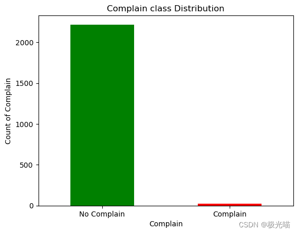
df['Complain'].value_counts()
# 1 if customer complained in the last 2 years, 0 otherwise

0    2219
1      21
Name: Complain, dtype: int64

• 从上图可以看出，顾客的投诉并不多。

# 让我们检查一下响应

# 响应：如果客户在最近 2 次活动中接受了优惠，则为 1，否则为 0
label_response = ["Denied","Accepted"]

count_response = pd.value_counts(df['Response'], sort=True)
count_response.plot(kind='bar', rot=0,color=['Green','Red'])
plt.title("Reponse class Distribution")
plt.xticks(range(2),label_response)
plt.xlabel("Respons")
plt.ylabel("Count of Response")

Text(0, 0.5, 'Count of Response')

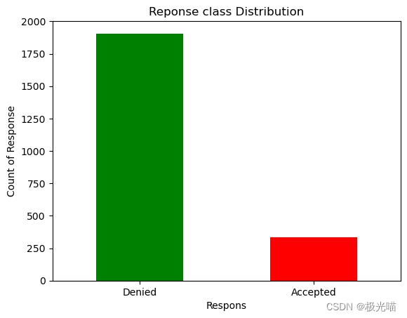
df['Response'].value_counts()

0    1906
1     334
Name: Response, dtype: int64

• 此图显示最后的优惠已被大多数客户拒绝

查看所有情况

• AcceptedCmp1：如果客户在第一个活动中接受了优惠，则为 1，否则为 0
• AcceptedCmp2：如果客户在第二次活动中接受了优惠，则为 1，否则为 0
• AcceptedCmp3：如果客户在第三次活动中接受了优惠，则为 1，否则为 0
• AcceptedCmp4：如果客户在第四次活动中接受了优惠，则为 1，否则为 0
• AcceptedCmp5：如果客户在第五次活动中接受了优惠，则为 1，否则为 0
• 响应：如果客户在上次活动中接受了优惠，则为 1，否则为 0

#Campagin 1

labels_c1 = ["Denied", "Accepted"]

count_c1 = pd.value_counts(df['AcceptedCmp1'], sort=True)
count_c1.plot(kind='bar', rot=0,color=['Green','Red'])
plt.title("AcceptedCmp1 class Distribution")
plt.xticks(range(2),labels_c1)
plt.xlabel("Campaign 1")
plt.ylabel("Count of Campagin1")

Text(0, 0.5, 'Count of Campagin1')

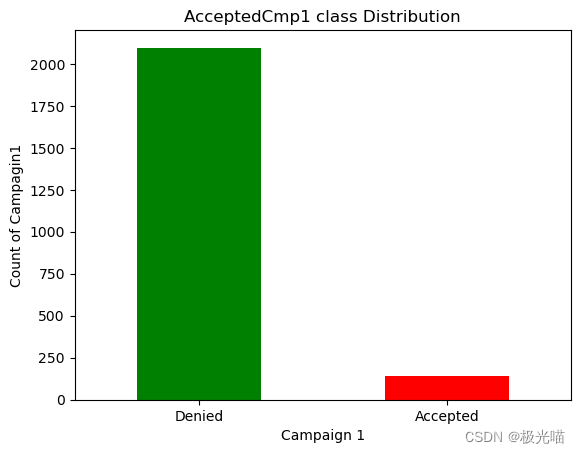
df['AcceptedCmp1'].value_counts()

0    2096
1     144
Name: AcceptedCmp1, dtype: int64

#Campagin 2

labels_c2 = ["Denied", "Accepted"]

count_c2 = pd.value_counts(df['AcceptedCmp2'], sort=True)
count_c2.plot(kind='bar', rot=0,color=['Green','Red'])
plt.title("AcceptedCmp2 class Distribution")
plt.xticks(range(2),labels_c2)
plt.xlabel("Campaign 2")
plt.ylabel("Count of Campagin2")

Text(0, 0.5, 'Count of Campagin2')

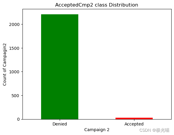
df["AcceptedCmp2"].value_counts()

0    2210
1      30
Name: AcceptedCmp2, dtype: int64

#Campagin 3

labels_c3 = ["Denied", "Accepted"]

count_c3 = pd.value_counts(df['AcceptedCmp3'], sort=True)
count_c3.plot(kind='bar', rot=0,color=['Green','Red'])
plt.title("AcceptedCmp3 class Distribution")
plt.xticks(range(2),labels_c3)
plt.xlabel("Campaign 3")
plt.ylabel("Count of Campagin3")

Text(0, 0.5, 'Count of Campagin3')

df["AcceptedCmp3"].value_counts()

0    2077
1     163
Name: AcceptedCmp3, dtype: int64

#Campagin 4

labels_c4 = ["Denied", "Accepted"]

count_c4 = pd.value_counts(df['AcceptedCmp4'], sort=True)
count_c4.plot(kind='bar', rot=0,color=['Green','Red'])
plt.title("AcceptedCmp4 class Distribution")
plt.xticks(range(2),labels_c4)
plt.xlabel("Campaign 4")
plt.ylabel("Count of Campagin4")

Text(0, 0.5, 'Count of Campagin4')

df["AcceptedCmp4"].value_counts()

0    2073
1     167
Name: AcceptedCmp4, dtype: int64

活动接受度比较。

• 从上面的数据我们可以清楚地看到，所有活动中的大部分优惠都被顾客拒绝了。
• 但活动 4 的接受度更高。
• 活动 4 > 活动 3 > 活动 1 > 活动 2

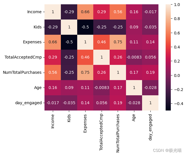
#Finding the correlation between the feature column

plt.figure(figsize=(20,18))
sns.heatmap(df.corr(), annot=True)
plt.show()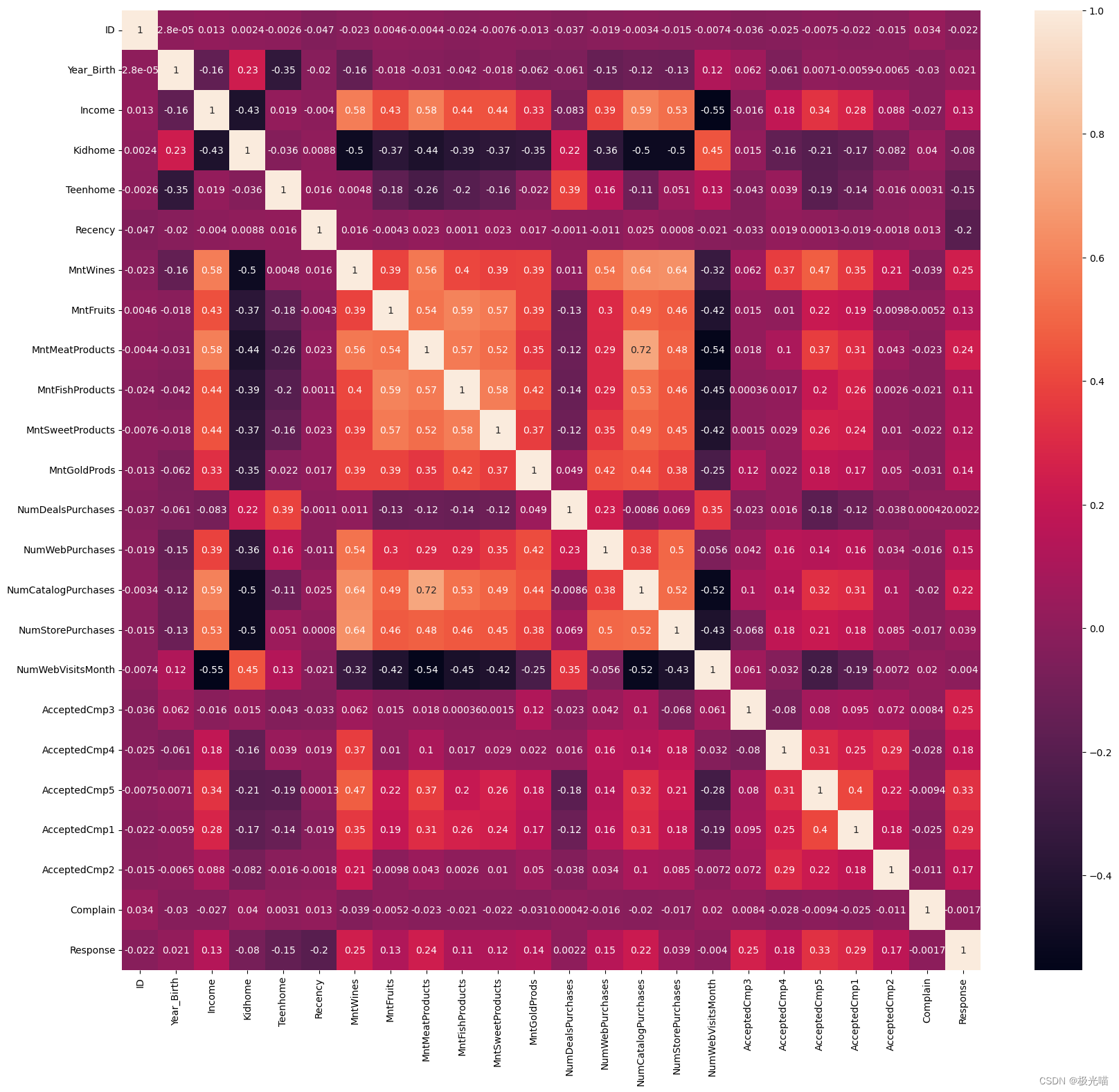

• 没有两列彼此有太多相关性，因此我们不能删除任何列

数据预处理

# Filling the missing value in the income by mean
df['Income'] = df['Income'].fillna(df['Income'].mean())
df.isnull().sum()

ID                     0
Year_Birth             0
Education              0
Marital_Status         0
Income                 0
Kidhome                0
Teenhome               0
Dt_Customer            0
Recency                0
MntWines               0
MntFruits              0
MntMeatProducts        0
MntFishProducts        0
MntSweetProducts       0
MntGoldProds           0
NumDealsPurchases      0
NumWebPurchases        0
NumCatalogPurchases    0
NumStorePurchases      0
NumWebVisitsMonth      0
AcceptedCmp3           0
AcceptedCmp4           0
AcceptedCmp5           0
AcceptedCmp1           0
AcceptedCmp2           0
Complain               0
Response               0
dtype: int64

• 数据集中没有空值

df.head()

	ID	Year_Birth	Education	Marital_Status	Income	Kidhome	Teenhome	Dt_Customer	Recency	MntWines	...	NumCatalogPurchases	NumStorePurchases	NumWebVisitsMonth	AcceptedCmp3	AcceptedCmp4	AcceptedCmp5	AcceptedCmp1	AcceptedCmp2	Complain	Response
0	5524	1957	Graduation	Single	58138.0	0	0	04-09-2012	58	635	...	10	4	7	0	0	0	0	0	0	1
1	2174	1954	Graduation	Single	46344.0	1	1	08-03-2014	38	11	...	1	2	5	0	0	0	0	0	0	0
2	4141	1965	Graduation	Together	71613.0	0	0	21-08-2013	26	426	...	2	10	4	0	0	0	0	0	0	0
3	6182	1984	Graduation	Together	26646.0	1	0	10-02-2014	26	11	...	0	4	6	0	0	0	0	0	0	0
4	5324	1981	PhD	Married	58293.0	1	0	19-01-2014	94	173	...	3	6	5	0	0	0	0	0	0	0

5 rows × 27 columns

# 检查“Marital_Status”中存在的唯一类别的数量

df['Marital_Status'].value_counts()

Married     864
Together    580
Single      480
Divorced    232
Widow        77
Alone         3
Absurd        2
YOLO          2
Name: Marital_Status, dtype: int64

df['Marital_Status'] = df['Marital_Status'].replace(['Married', 'Together'],'relationship')
df['Marital_Status'] = df['Marital_Status'].replace(['Divorced', 'Widow', 'Alone', 'YOLO', 'Absurd','single'],'Single')

• 在上面的单元格中，我们将“已婚”、“在一起”分组为“关系”
• 而“离婚”、“寡妇”、“孤独”、“YOLO”、“荒谬”则为“单身”

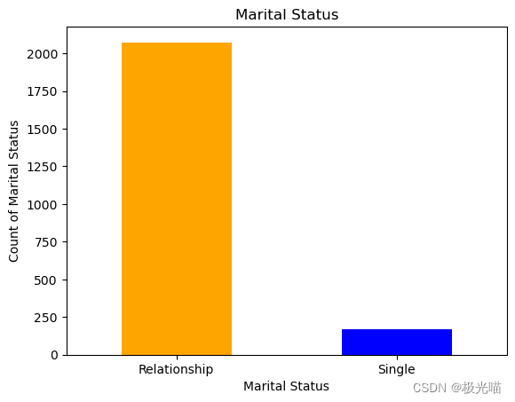
df['Marital_Status'].value_counts()

relationship    1444
Single           796
Name: Marital_Status, dtype: int64

# Relationship vs Single

labels_status = ["Relationship", "Single"]

count_status = pd.value_counts(df['Marital_Status'], sort=True)
count_c4.plot(kind='bar', rot=0,color=['Orange','Blue'])
plt.title("Marital Status")
plt.xticks(range(2),labels_status)
plt.xlabel("Marital Status")
plt.ylabel("Count of Marital Status")

Text(0, 0.5, 'Count of Marital Status')

将不同的数据帧组合成一列以减少维数

df['Kids'] = df['Kidhome'] + df['Teenhome']
df['Expenses'] = df['MntWines'] + df['MntFruits'] + df['MntMeatProducts'] + df['MntFishProducts'] + df['MntSweetProducts'] + df['MntGoldProds']
df['TotalAcceptedCmp'] = df['AcceptedCmp1'] + df['AcceptedCmp2'] + df['AcceptedCmp3'] + df['AcceptedCmp4'] + df['AcceptedCmp5'] + df['Response']
df['NumTotalPurchases'] = df['NumWebPurchases'] + df['NumCatalogPurchases'] + df['NumStorePurchases'] + df['NumDealsPurchases']

#保存表格数据
df.to_csv('data_visuals.csv')

# 删除一些列以减少模型的维度和复杂性
col_del = ["AcceptedCmp1" , "AcceptedCmp2", "AcceptedCmp3" , "AcceptedCmp4","AcceptedCmp5", "Response","NumWebVisitsMonth", "NumWebPurchases","NumCatalogPurchases","NumStorePurchases","NumDealsPurchases" , "Kidhome", "Teenhome","MntWines", "MntFruits", "MntMeatProducts", "MntFishProducts", "MntSweetProducts", "MntGoldProds"]
df=df.drop(columns=col_del,axis=1)
df.head()

	ID	Year_Birth	Education	Marital_Status	Income	Dt_Customer	Recency	Complain	Kids	Expenses	TotalAcceptedCmp	NumTotalPurchases
0	5524	1957	Graduation	Single	58138.0	04-09-2012	58	0	0	1617	1	25
1	2174	1954	Graduation	Single	46344.0	08-03-2014	38	0	2	27	0	6
2	4141	1965	Graduation	relationship	71613.0	21-08-2013	26	0	0	776	0	21
3	6182	1984	Graduation	relationship	26646.0	10-02-2014	26	0	1	53	0	8
4	5324	1981	PhD	relationship	58293.0	19-01-2014	94	0	1	422	0	19

# Adding 'Age' column

df['Age'] = 2015 - df['Year_Birth']

df['Education'].value_counts()

Graduation    1127
PhD            486
Master         370
2n Cycle       203
Basic           54
Name: Education, dtype: int64

# 仅将类别更改为 UG 和 PG

df['Education'] = df['Education'].replace(['PhD','2n Cycle','Graduation', 'Master'],'PG')  
df['Education'] = df['Education'].replace(['Basic'], 'UG')

# 客户与公司互动的天数

# 将 bt_customer 更改为时间戳格式
df['Dt_Customer'] = pd.to_datetime(df.Dt_Customer)
df['first_day'] = '01-01-2015'
df['first_day'] = pd.to_datetime(df.first_day)
df['day_engaged'] = (df['first_day'] - df['Dt_Customer']).dt.days

df=df.drop(columns=["ID", "Dt_Customer", "first_day", "Year_Birth", "Dt_Customer", "Recency", "Complain"],axis=1)
df.shape

(2240, 9)

df.head()

	Education	Marital_Status	Income	Kids	Expenses	TotalAcceptedCmp	NumTotalPurchases	Age	day_engaged
0	PG	Single	58138.0	0	1617	1	25	58	997
1	PG	Single	46344.0	2	27	0	6	61	151
2	PG	relationship	71613.0	0	776	0	21	50	498
3	PG	relationship	26646.0	1	53	0	8	31	91
4	PG	relationship	58293.0	1	422	0	19	34	347

数据可视化

fig = px.bar(df, x='Marital_Status', y='Expenses', color="Marital_Status")
fig.show()

# Less number of single customer
fig = px.histogram (df, x = "Expenses",  facet_row = "Marital_Status",  template = 'plotly_dark')
fig.show ()

fig = px.histogram (df, x = "Expenses",  facet_row = "Education",  template = 'plotly_dark')
fig.show ()

fig = px.histogram (df, x = "NumTotalPurchases",  facet_row = "Education",  template = 'plotly_dark')
fig.show ()

fig = px.histogram (df, x = "Age",  facet_row = "Marital_Status",  template = 'plotly_dark')
fig.show ()

fig = px.histogram (df, x = "Income",  facet_row = "Marital_Status",  template = 'plotly_dark')
fig.show ()

fig =  px.pie (df, names = "Marital_Status", hole = 0.4, template = "gridon")
fig.show ()

• 35% 的客户是单身，而 64% 的客户是恋爱中的客户。

fig =  px.pie (df, names = "Education", hole = 0.4, template = "plotly_dark")
fig.show ()

• 超过97%的客户来自PG背景。 和大约。 2%来自UG。

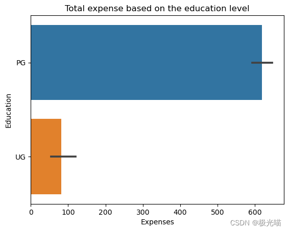
sns.barplot(x=df['Expenses'], y=df['Education'])
plt.title('Total expense based on the education level')

Text(0.5, 1.0, 'Total expense based on the education level')

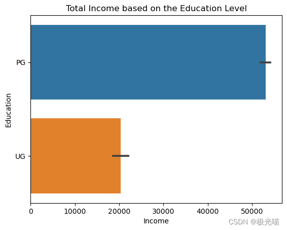
sns.barplot(x=df['Income'], y=df['Education'])
plt.title('Total Income based on the Education Level')

Text(0.5, 1.0, 'Total Income based on the Education Level')

df.describe()

	Income	Kids	Expenses	TotalAcceptedCmp	NumTotalPurchases	Age	day_engaged
count	2240.000000	2240.000000	2240.000000	2240.000000	2240.000000	2240.000000	2240.000000
mean	52247.251354	0.950446	605.798214	0.446875	14.862054	46.194196	538.043304
std	25037.797168	0.751803	602.249288	0.890543	7.677173	11.984069	232.229893
min	1730.000000	0.000000	5.000000	0.000000	0.000000	19.000000	26.000000
25%	35538.750000	0.000000	68.750000	0.000000	8.000000	38.000000	366.750000
50%	51741.500000	1.000000	396.000000	0.000000	15.000000	45.000000	539.000000
75%	68289.750000	1.000000	1045.500000	1.000000	21.000000	56.000000	711.250000
max	666666.000000	3.000000	2525.000000	5.000000	44.000000	122.000000	1089.000000

sns.heatmap(df.corr(),annot=True)

<Axes: >

obj = []
for i in df.columns:
    if(df[i].dtypes=="object"):
        obj.append(i)

print(obj)

['Education', 'Marital_Status']

# Label Encoding
from sklearn.preprocessing import LabelEncoder

df['Marital_Status'].value_counts()

relationship    1444
Single           796
Name: Marital_Status, dtype: int64

lbl_encode = LabelEncoder()
for i in obj:
    df[i] = df[[i]].apply(lbl_encode.fit_transform)

df1 = df.copy()
df1.head()

	Education	Marital_Status	Income	Kids	Expenses	TotalAcceptedCmp	NumTotalPurchases	Age	day_engaged
0	0	0	58138.0	0	1617	1	25	58	997
1	0	0	46344.0	2	27	0	6	61	151
2	0	1	71613.0	0	776	0	21	50	498
3	0	1	26646.0	1	53	0	8	31	91
4	0	1	58293.0	1	422	0	19	34	347

数据标准化

from sklearn.preprocessing import StandardScaler

scaled_features = StandardScaler().fit_transform(df1.values)
scaled_features_df = pd.DataFrame(scaled_features, index=df1.index, columns=df1.columns)

scaled_features_df.head()

	Education	Marital_Status	Income	Kids	Expenses	TotalAcceptedCmp	NumTotalPurchases	Age	day_engaged
0	-0.157171	-1.346874	0.235327	-1.264505	1.679417	0.621248	1.320826	0.985345	1.976745
1	-0.157171	-1.346874	-0.235826	1.396361	-0.961275	-0.501912	-1.154596	1.235733	-1.667011
2	-0.157171	0.742460	0.773633	-1.264505	0.282673	-0.501912	0.799685	0.317643	-0.172468
3	-0.157171	0.742460	-1.022732	0.065928	-0.918094	-0.501912	-0.894025	-1.268149	-1.925433
4	-0.157171	0.742460	0.241519	0.065928	-0.305254	-0.501912	0.539114	-1.017761	-0.822831

肘部法则确定聚类数量

from sklearn.cluster import KMeans

wcss = []
for i in range(1,11):
    kmeans = KMeans(n_clusters=i, init='k-means++', random_state=42)
    kmeans.fit(scaled_features_df)
    wcss.append(kmeans.inertia_)
    # inetia_: Sum of squared distances of samples to their closest cluster center, weighted by the sample weights if provided.
plt.figure(figsize=(16,8))
plt.plot(range(1,11), wcss, 'bx-')
plt.title('The Elbow Maethod')
plt.xlabel('Number of Clusters')
plt.ylabel('WCSS')
plt.show()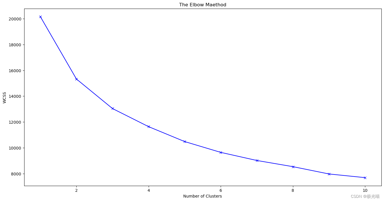

拐点不清晰，肘法中并不太清楚应该选择哪个K值

剪影系数

from sklearn.metrics import silhouette_score

silhouette_scores = []
for i in range(2,10):
    m1 = KMeans(n_clusters=i, random_state=42)
    c = m1.fit_predict(scaled_features_df)
    silhouette_scores.append(silhouette_score(scaled_features_df, m1.fit_predict(scaled_features_df)))
    
plt.bar(range(2,10), silhouette_scores)
plt.xlabel('Number of clusters', fontsize=20)
plt.ylabel('S(i)', fontsize=20)
plt.show()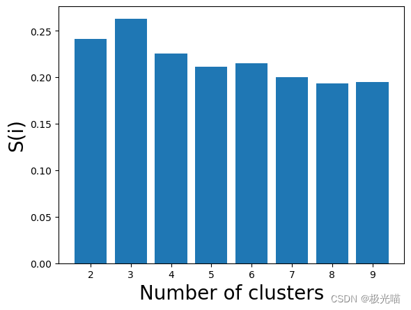

# 现在我们用Silhouette Score来衡量K的值
silhouette_scores

[0.24145101432627075,
 0.2630066765900862,
 0.22547869857815794,
 0.2112495373878677,
 0.2149228429852001,
 0.1997135405176978,
 0.19301680336746188,
 0.19495794809915995]

# 获取轮廓分数的最大值并在索引中添加2 因为索引从2开始

sc = max(silhouette_scores)
num_of_clusters = silhouette_scores.index(sc)+2
print("Number of Cluster Required is: ", num_of_clusters)

Number of Cluster Required is:  3

建立模型

# 使用 K 均值算法训练预测。

kmeans = KMeans(n_clusters = num_of_clusters, random_state=42).fit(scaled_features_df)
pred = kmeans.predict(scaled_features_df)

pred

array([1, 0, 1, ..., 1, 1, 0])

# 添加这些聚类值到 main dataframe (without standardization)中
df['cluster'] = pred + 1

df.head()

	Education	Marital_Status	Income	Kids	Expenses	TotalAcceptedCmp	NumTotalPurchases	Age	day_engaged	cluster
0	0	0	58138.0	0	1617	1	25	58	997	2
1	0	0	46344.0	2	27	0	6	61	151	1
2	0	1	71613.0	0	776	0	21	50	498	2
3	0	1	26646.0	1	53	0	8	31	91	1
4	0	1	58293.0	1	422	0	19	34	347	1

# 保存数据
df.to_csv('data_visuals2.csv')

pl = sns.countplot(x=df["cluster"])
pl.set_title("Distribution Of The Clusters")
plt.show()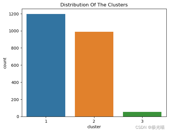

正如我们在这里看到的，与其他聚类相比，聚类 1 中的权重更大。

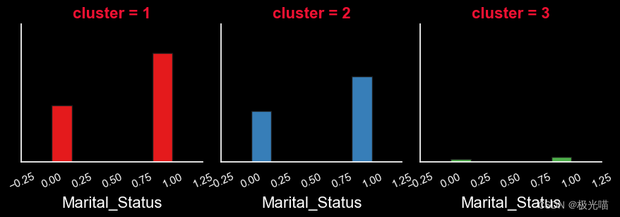
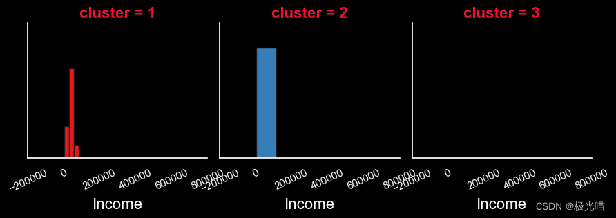
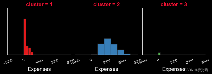
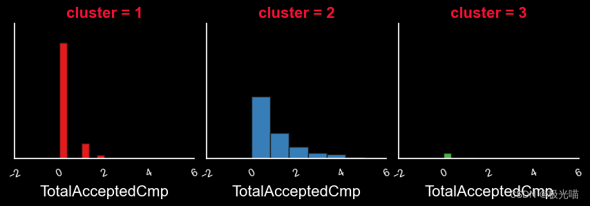
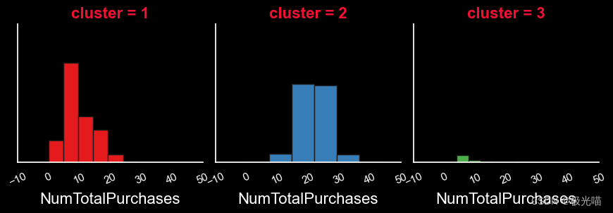
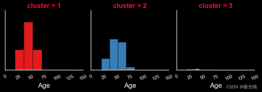
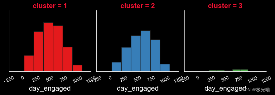
sns.set(rc={'axes.facecolor':'black', 'figure.facecolor':'black', 'axes.grid' : False}) 
for i in df:
    diag = sns.FacetGrid(df, col="cluster", hue="cluster", palette="Set1")
    diag.map(plt.hist, i, bins=6, ec="k") 
    diag.set_xticklabels(rotation=25, color='white')
    diag.set_yticklabels(color='white')
    diag.set_xlabels(size=16, color='white')
    diag.set_titles(size=16, color='#f01132', fontweight="bold")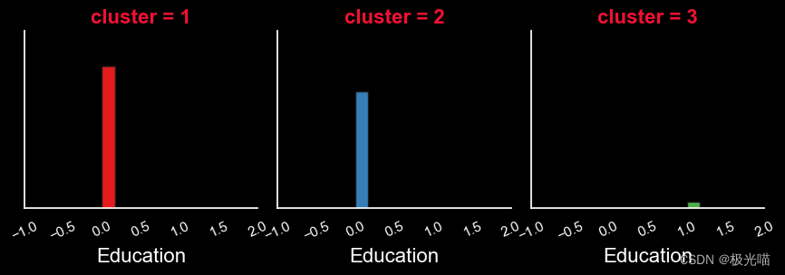

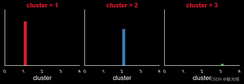
报告

根据以上信息，我们可以将客户分为三部分：-

1. 高度活跃客户：这些客户属于集群一。
2. 中等活跃客户：- 这些客户属于集群二。
3. 最不活跃的客户 ：- 这些客户属于第三集群。

高度活跃客户的特征

• 在教育方面

  • 高活跃客户来自PG背景

• 就婚姻状况而言

  • 恋爱关系中的人数约为。 单身人士的两倍

• 就收入而言

  • 高度活跃客户的收入略低于中等活跃客户。

• 就孩子而言

  • 与其他顾客相比，高度活跃的顾客拥有更多的孩子（平均 1 个孩子）。

• 就费用而言

  • 高度活跃客户的费用低于中等客户。
  • 这些客户的平均花费。 约。 100-200单位钱。

• 就年龄而言

  • 这些顾客的年龄在25岁至75岁之间。
  • 顾客年龄上限为 40 至 50 岁。

• 就参与天数而言

  • 高度活跃的客户由于与公司接触的时间较长而更加忠诚。

中等活跃客户的特征

• 在教育方面

  • 中等活跃客户也来自PG背景

• 就婚姻状况而言

  • 与单身人士相比，恋爱中的人数略多。

• 就收入而言

  • 中等活跃客户的收入高于其他客户。

• 就孩子而言

  • 与高度活跃的客户相比，中等活跃的客户的子女数量较少（最多客户没有子女）。

• 就费用而言

  • 与活跃客户相比，中等活跃客户的费用更高。
  • 这些客户的平均花费。 约。 500-2000单位钱。

• 就年龄而言

  • 这些顾客的年龄在25岁至75岁之间。
  • 顾客年龄上限为 35 至 60 岁。

• 就参与天数而言

  • 与高度活跃的客户相比，中等活跃的客户与公司的互动程度略低

 代码与数据集下载

详情请见顾客喜好分析项目（用户画像）-VenusAI (aideeplearning.cn)