【OpenCV实践之】描述符BEBLID
目录BEBLID简介BEBLID论文浅述C++代码部分实验结果小结参考文献BEBLID简介 局部特征描述子基本停滞许久没有出现新的算法,最近看到OpenCV-4.5.1集成了一个新的二进制描述子。BEBLID(Boosted efficient binary local image descriptor)在速度上面与精度上面要优于ORB算法。应用过相关ORB算法都知道,ORB算法由于其速度卓同时
BEBLID简介
局部特征描述子基本停滞许久没有出现新的算法,最近看到OpenCV-4.5.1集成了一个新的二进制描述子。BEBLID(Boosted efficient binary local image descriptor)在速度上面与精度上面要优于ORB算法。应用过相关ORB算法都知道,ORB算法由于其速度卓同时匹配性能很高而得名,广泛应用于工业界。那么,现在出现BEBLID描述子,匹配成功率高于ORB几乎能够媲美SIFT算法,论文阐述不知道鲁棒性与SIFT相比如何。如果你安装的OpenCV版本大于等于4.5.1,那么可以通过编译对应的opencv_contirb来直接调用BEBLID,该描述子在cv::xfeature2d作用域下面。如果版本没有的话,那么可以在文末获取原作者的BEBLID的链接,来进行使用,比较容易。我的安装这么高版本OpenCV,同时我也阅读一个作者的源代码,并进行简单的运行分析效果。
BEBLID论文
关于BEBLID描述子的解释请参考这篇博文:BELID:增强的高效的局部图像描述符。如果侵权,请联系删除。
C++代码部分
这部分代码是直接调用OpenCV接口来显示匹配结果的代码,所以要使用的话建议先编译对于成功的opencv_contirb。python版本代码较为简单,可以参考文末链接②。特征点检测算子与描述符算子分开,使用used_beblid来是否调用BEBLID描述子。调用OpenCV的API代码也比较简单,与之前的MSER或者DAISY类似,如有兴趣请参考我之前的博客。
#include <iostream>
#include <opencv2/opencv.hpp>
#include <opencv2/xfeatures2d.hpp>

/**
 * This demo shows how BEBLID descriptor can be used with a feature detector (here ORB) to
 * detect, describe and match two images of the same scene.
 */
int main()
{
	// Read the input images in grayscale format (CV_8UC1)
	cv::Mat img1 = cv::imread("./imgs/img1.jpg", cv::IMREAD_GRAYSCALE);
	cv::Mat img2 = cv::imread("./imgs/img3.jpg", cv::IMREAD_GRAYSCALE);

	bool used_beblid = false; // true: beblid  false: brief

	// Create the feature detector, for example ORB
	auto detector = cv::ORB::create();

	// Use 32 bytes per descriptor and configure the scale factor for ORB detector
	auto beblid = cv::xfeatures2d::BEBLID::create(0.75, cv::xfeatures2d::BEBLID::SIZE_256_BITS);
	auto brief  = cv::xfeatures2d::BriefDescriptorExtractor::create(32, true);
	// Detect features in both images
	std::vector<cv::KeyPoint> points1, points2;
	detector->detect(img1, points1);
	detector->detect(img2, points2);
	std::cout << "Detected  " << points1.size() << " kps in image1" << std::endl;
	std::cout << "Detected  " << points2.size() << " kps in image2" << std::endl;
	//// Describe the detected features i both images
	cv::Mat descriptors1, descriptors2;

	if (used_beblid)
	{
		beblid->compute(img1, points1, descriptors1);
		beblid->compute(img2, points2, descriptors2);
	}
	else
	{
		//detector->compute(img1, points1, descriptors1);
		//detector->compute(img2, points2, descriptors2);
		brief->compute(img1, points1, descriptors1);
		brief->compute(img2, points2, descriptors2);
	}
	std::cout << "Points described" << std::endl;

	// Match the generated descriptors for img1 and img2 using brute force matching
	cv::BFMatcher matcher(cv::NORM_HAMMING, true);
	std::vector<cv::DMatch> matches;
	matcher.match(descriptors1, descriptors2, matches);
	std::cout << "Number of matches: " << matches.size() << std::endl;

	// If there is not enough matches exit
	if (matches.size() < 4)
		exit(-1);

	// Take only the matched points that will be used to calculate the
	// transformation between both images
	std::vector<cv::Point2d> matched_pts1, matched_pts2;
	for (cv::DMatch match : matches)
	{
		matched_pts1.push_back(points1[match.queryIdx].pt);
		matched_pts2.push_back(points2[match.trainIdx].pt);
	}

	// Find the homography that transforms a point in the first image to a point in the second image.
	cv::Mat inliers;
	cv::Mat H = cv::findHomography(matched_pts1, matched_pts2, cv::RANSAC, 3, inliers);
	// Print the number of inliers, that is, the number of points correctly
	// mapped by the transformation that we have estimated
	std::cout << "Number of inliers " << cv::sum(inliers)[0]
		<< " ( " << (100.0f * cv::sum(inliers)[0] / matches.size()) << "% )" << std::endl;

	// Convert the image to BRG format from grayscale
	cv::cvtColor(img1, img1, cv::COLOR_GRAY2BGR);
	cv::cvtColor(img2, img2, cv::COLOR_GRAY2BGR);

	// Draw all the matched keypoints in red color
	cv::Mat all_matches_img;
	cv::drawMatches(img1, points1, img2, points2, matches, all_matches_img,
		CV_RGB(255, 0, 0), CV_RGB(255, 0, 0));  // Red color

	// Draw the inliers in green color
	for (int i = 0; i < matched_pts1.size(); i++)
	{
		if (inliers.at<uchar>(i, 0))
		{
			cv::circle(all_matches_img, matched_pts1[i], 3, CV_RGB(0, 255, 0), 2);
			// Calculate second point assuming that img1 and img2 have the same height
			cv::Point p2(matched_pts2[i].x + img1.cols, matched_pts2[i].y);
			cv::circle(all_matches_img, p2, 3, CV_RGB(0, 255, 0), 2);
			cv::line(all_matches_img, matched_pts1[i], p2, CV_RGB(0, 255, 0), 2);
		}
	}

	// Show and save the result
	cv::imshow("All matches", all_matches_img);
	cv::imwrite("./imgs/inliners_img.jpg", all_matches_img);

	// Transform the first image to look like the second one
	cv::Mat transformed;
	cv::warpPerspective(img1, transformed, H, img2.size());
	cv::imshow("Original image", img2);
	cv::imshow("Transformed image", transformed);

	cv::waitKey(0);

	return 0;
}
实验结果
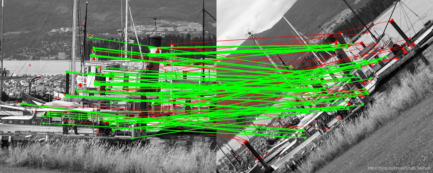
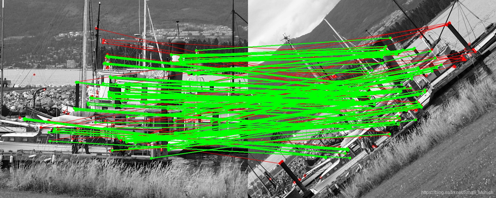
下面表格对比ORB检测算子基础上,BRIEF与BRBLID描述子的性能与鲁棒性。明显可以看到BEBLID描述子要优于BRIEF描述子,最后一个ORB是直接使用OpenCV集成的ORB算法进行检测与描述符,性能优于上述两种。目前我觉得有些诧异,查看源码部分发现并没有什么改变,OpenCV集成的ORB算法与本文上面单独构建BRIEF描述子按道理应该一致。
| 算法 | 匹配点(个) | 内联点(个) | 匹配率(百分比) |
|---|---|---|---|
| ORB + BRIEF | 156 | 96 | 61.5385% |
| ORB + BEBLID | 228 | 172 | 75.4388% |
| ORB | 238 | 185 | 77.7311% |
下面贴一下匹配的示例图结果:

小结
特征检测与描述当下已经很少做此方面的研究,很高兴2020年还能够由此文章发布,并且被OpenCV代码集成,说明此算法很有工程意义。忽然间,我想到要是把检测模块、描述符模块、匹配模块是否可以组合出一个最强的匹配算法兼顾性能与效率的情况下。检测模块:最先出现且工业应用ORB算法,或者加速版本SURF,描述符目前BEBLID与加速版SURF,匹配策略让我想到FLANN匹配,同时经匹配阶段的GMS都是优秀的算法,同时也被OpenCV所集成。well,如果你感兴趣可以试着组合其中各个算法来看看效果。
参考文献

有“AI”的1024 = 2048,欢迎大家加入2048 AI社区
更多推荐


 7
7 0
0- 0


 已为社区贡献12条内容

所有评论(0)