论文题目：Learning Deep Features for Discriminative Localization
(Class Activation Mapping)
论文地址：https://arxiv.org/pdf/1512.04150.pdf
完整代码：https://github.com/metalbubble/CAM
—————————————————————————————————

论文研读

问题：
1.以前的全监督的CNN方法，会进行标签标注，导致浪费大量的人力与时间成本。

2.全连接层
a) 全连接层被用作分类，所以导致在此层的定位能力丢失（卷积神经网络的全连接层会将最后一层的特征图拉平，这样空间位置信息就破坏了，而全局平均池化层不会破坏空间结构）。
b) 全连接层有大量参数，计算成本高。

主要贡献：
1.使用弱监督目标定位
2.CNN内部表示的可视化

流程图: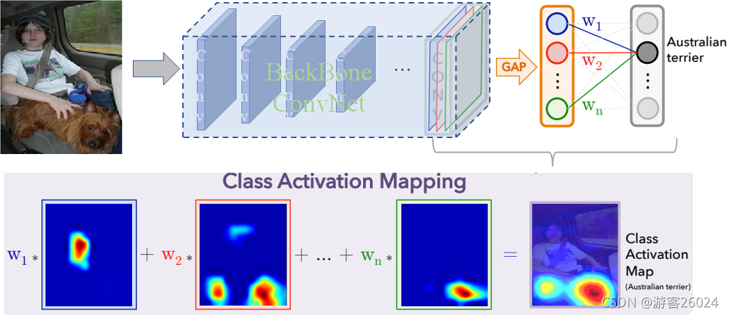
方法：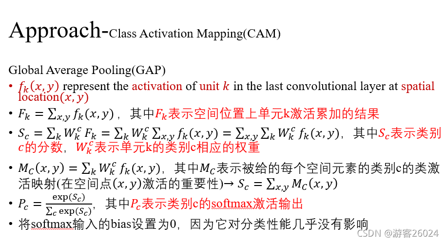

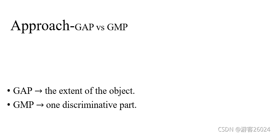
使用全局平均池化GAP（Global Average Pooling）与GMP（Global Max Pooling）的区别：
GMP能够帮助卷积神经网络找到一个不同的区域，而GAP则能够精确的找到目标在图像中的范围。对于GAP来说，所有较高的值都会对整体训练有比较大的贡献（取平均值）。对于GMP来说，只有最大值的那个点会产生贡献。作者在ImageNet 上测试了两种全局池化方式，发现分类结果相近，但是定位的结果GAP远远超过GMP。

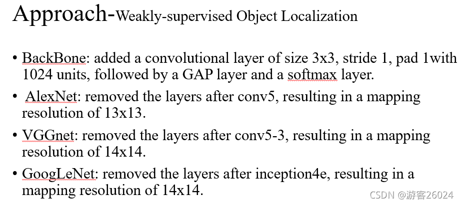
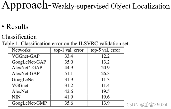
从表1可得，我们的分类error相对于使用全连接层的error来说，相差1-2个百分点。比如VGGnet 31.2 top1 error vs VGGnet-GAP 33.4 top1 error| AlexNet 42.6 top1 error vs AlexNet*-GAP 44.9 top1 error (加*代表在替换fc层之后，又增加2层卷积层，再加了GAP层)。我们GAP的分类结果相比与GMP分类来说，效果更好（理由如上）。

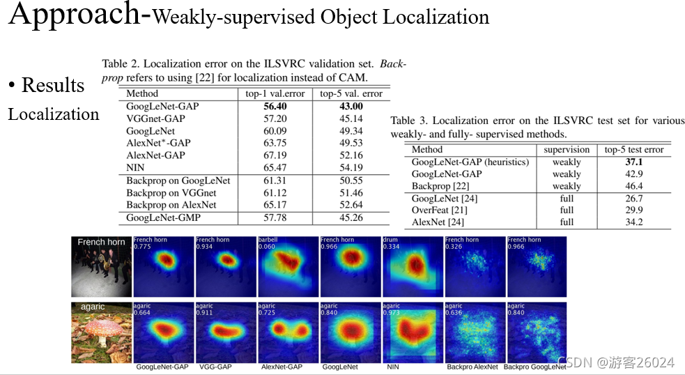
从表2可得，我们使用全局平均池化的方法定位 比 反向传播的CNN方法定位、全局最大池化的方法定位 效果更好，其中GoogLeNet-GAP最佳为56.40 top1 error | 43.00 top5 error

从表3可得，我们使用的弱监督定位方法 比 全监督定位方法 想过更好，其中GoogLeNet-GAP(启发式 [修改了 bbox] ) 为 37.1 top5 error

上图表示，每个BackBone 生成的不同定位方法，使用热力图展示，其中BackBone的VGG-GAP效果最好。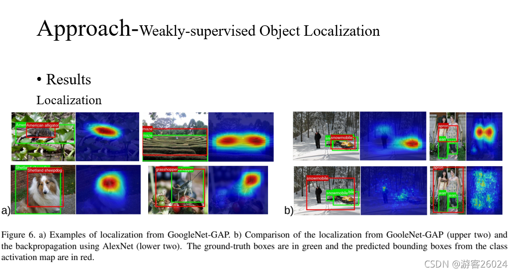

从图6可得，其中在原图上现实的绿框为Ground Truth,红框为预测的结果。a)为使用BackBone（GooLeNet-GAP）的结果，b)为GoogLeNet-GAP（upper two）与 the backpropagation using AlexNet (lower two)的结果。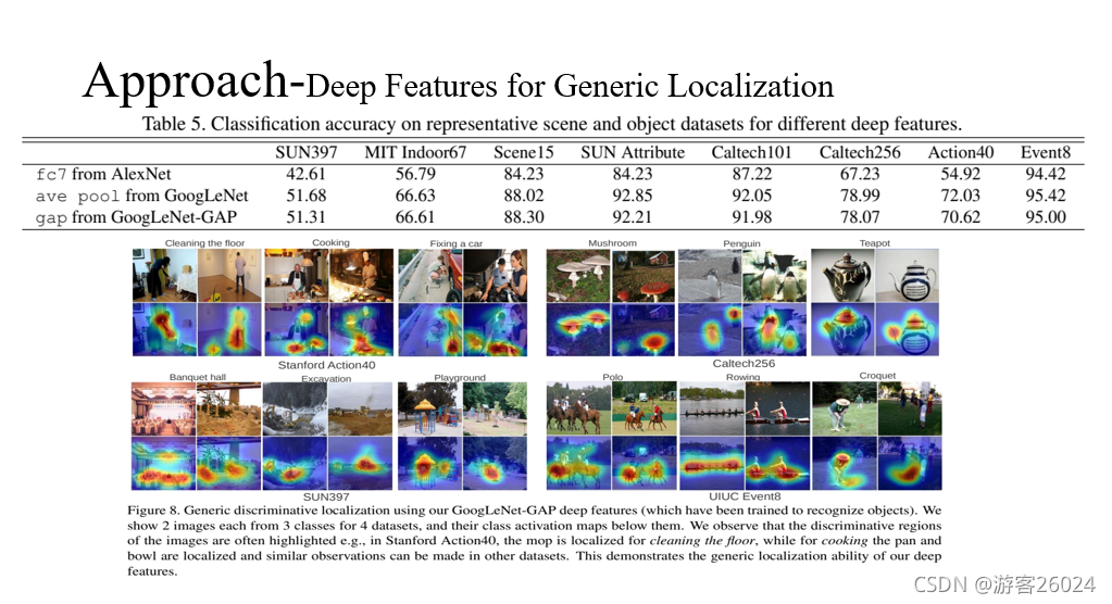

从表5可得，使用不同的数据集与BackBone产生的精度结果。

从图8可得，使用不同数据集与GoogLeNet-GAP产生的定位结果。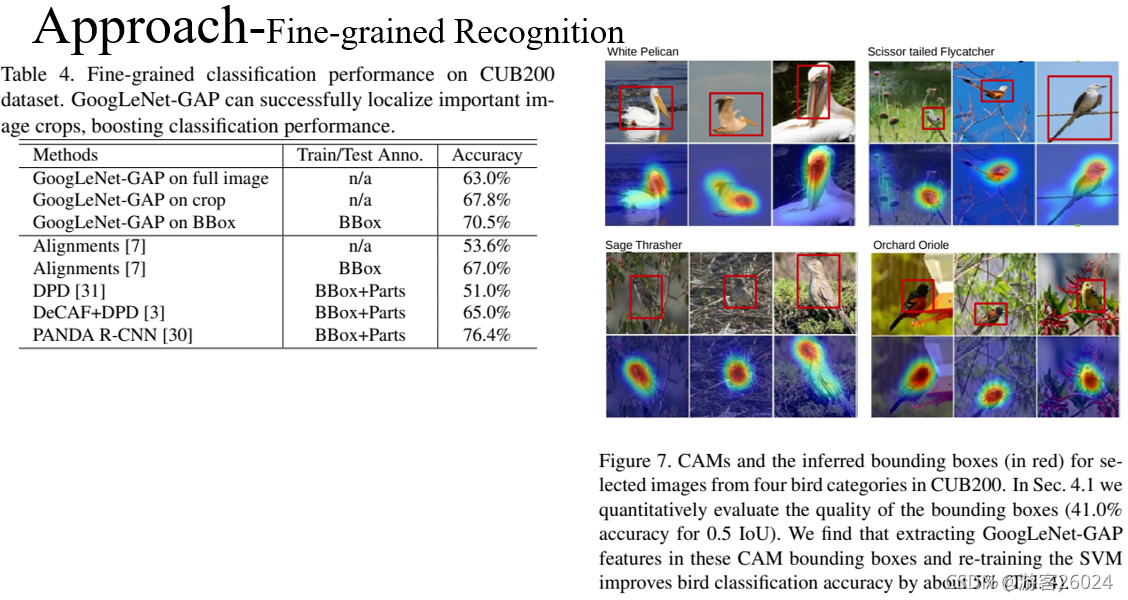

从表4可得，在CUB200数据集与GoogLeNet-GAP产生的细粒度分类性能，并能成功定位重要图像区域。

从图7可得，使用弱监督定位方法产生的bbox。

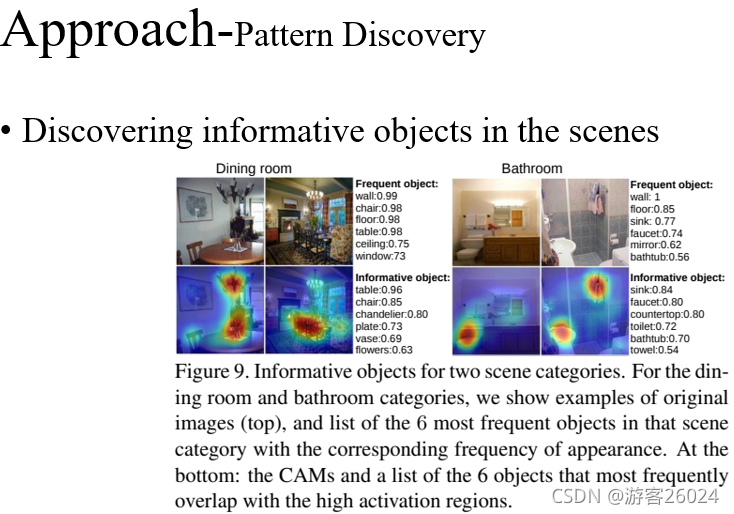
从图9可得，不同场景下的带信息的目标效果。

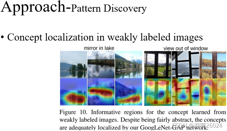
从图10可得，在弱标签图像的概念定位(镜子、湖等)。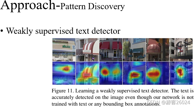

从图11可得，弱监督文本检测的结果。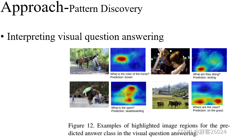

从图12可得，图像问答的定位结果。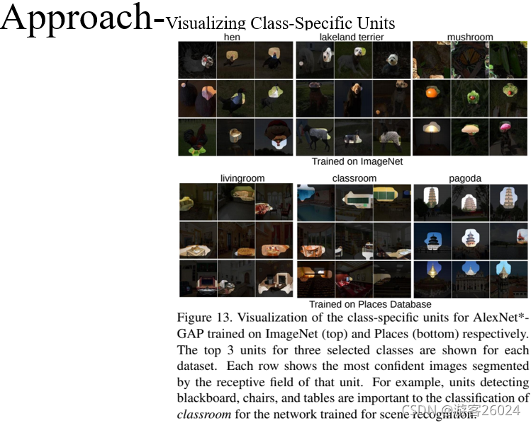

从图13可得，特殊类别单元的可视化，Mask结果。

—————————————————————————————————

代码复现

import os
import cv2
from PIL import Image
from torchvision import models, transforms
from torch.autograd import Variable
from torch.nn import functional as F
import numpy as np
from torchvision.models.densenet import densenet161
import json

# input image 
# 使用本地的图片与本地的标签
labels_file = 'imagenet-simple-labels.json'
image_path = "31.jpg"

# networks such as Googlenet, ResNet,Densent already use global average pooling at the end,
# so CAM could be used directly.

# 选择使用的网络
model_id = 2

# 选择网络
if model_id == 1:
    net = models.squeezenet1_1(pretrained=True)
    finalconv_name = 'features'

elif model_id == 2:
    net = models.resnet18(pretrained=True)
    finalconv_name = 'layer4'
elif model_id == 3:
    net = densenet161()
    finalconv_name = "features"

# 有固定参数作用，如norm的参数
net.eval()

# 获取特定层的feature map
# hook the feature extractor
features_blobs = []


def hook_feature(module, input, output):
    features_blobs.append(output.data.cpu().numpy())


net._modules.get(finalconv_name).register_forward_hook(hook_feature)

# get the softmax weight
# 倒数第二层
params = list(net.parameters()) # 将参数变换为列表
weight_softmax = np.squeeze(params[-2].data.numpy()) # 提取softmax层的参数

# 生成CAM图的函数，完成权重和feature相乘操作
def returnCAM(feature_conv, weight_softmax, class_idx):
    # generate the class activation maps upsample to 256x256
    size_upsample = (256, 256)
    bc, nc, h, w = feature_conv.shape
    output_cam = []
    # class_idx为预测分数较大的类别数字表示的数组，一张图片中有N个类物体，则数组中N个元素
    for idx in class_idx:
        # 回到GAP的值
        # weight_softmax中预测为第idx类的参数w乘以feature_map,为了相乘reshape map的形状
        cam = weight_softmax[idx].dot(feature_conv.reshape(nc, h * w))
        #将feature_map的形状reshape回去
        cam = cam.reshape(h, w)
				
				# 归一化操作（最小值为0，最大值为1）
        # np.min 返回数组的最小值或沿轴的最小值
        cam = cam - np.min(cam)
        cam_img = cam / np.max(cam)
			
				# 转换为图片255的数据
        # np.uint8() Create a data type object.
        cam_img = np.uint8(255 * cam_img)

			 # resize 图片尺寸与输入图片一致
        output_cam.append(cv2.resize(cam_img, size_upsample))

    return output_cam

# 数据处理，先缩放尺寸到(224,224)，再变换数据类型为tensor,最后normalize
normalize = transforms.Normalize(
    mean=[0.485, 0.456, 0.406],
    std=[0.229, 0.224, 0.225]
)

preprocess = transforms.Compose([
    transforms.Resize((224, 224)),
    transforms.ToTensor(),
    normalize
])
image_path = os.path.expanduser(image_path)
img_pil = Image.open(image_path)
img_pil.save('test.jpg')
# 将图片数据处理成所需要的可用数据 tensor
img_tensor = preprocess(img_pil)
# 处理图片为Variable数据
img_variable = Variable(img_tensor.unsqueeze(0))
#将图片输入网络得到预测类别分数
logit = net(img_variable)
# 分类标签列表，并存储在classes(数字类别，类别名称)
with open(labels_file) as f:
    classes = json.load(f)
    
# 使用softmax打分
h_x = F.softmax(logit, dim=1).data.squeeze()
# 对分类的预测类别分数排序，输出预测值和在列表中的位置
probs, idx = h_x.sort(0, True)

# 转换数据类型
probs = probs.numpy()
idx = idx.numpy()

# 输出预测分数排名在前5个类别的预测分数和对应的类别名称
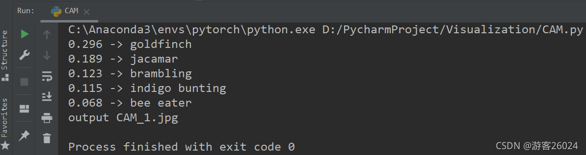
for i in range(0, 5):
    print('{:.3f} -> {}'.format(probs[i], classes[idx[i]]))

# 输出与图片尺寸一致的CAM图片
# generate class activation mapping for the top1 prediction
CAMs = returnCAM(features_blobs[0], weight_softmax, [idx[0]])

# render the CAM and output
print("output CAM.jpg")

# 将图片和CAM拼接在一起展示定位结果
img = cv2.imread("31.jpg")
height, width, _ = img.shape
# 生成热力图
heatmap = cv2.applyColorMap(cv2.resize(CAMs[0], (width, height)), cv2.COLORMAP_JET)
result = cv2.addWeighted(img, 0.3, heatmap, 0.5, 0)
cv2.imwrite('CAM.jpg', result)
cv2.imshow("heatmap", result)
cv2.waitKey(0)
cv2.destroyAllWindows()

注意：
1.本地标签的下载 点击我

2.使用残差网络作为BackBone，效果更好

效果展示
原图：
___________________________________________________________
CAM热力图展示：
___________________________________________________________

控制台现实最大的前五个类别的置信度：