---

前言

前面我们已经初步了解了 BP 神经网络的层级结构，以及其前向传播与反向传播的基本流程。接下来，以 MNIST 数据集为例，具体设计一个基础的神经网络(多层感知机)，并使用 Python 实现网络中的各个函数，同时搭配数据可视化以更清晰的理解网络的运作过程。

---

一、MNIST数据集

1.1 数据集说明

(1)数据集概要

• 数据量：70,000 张图片
• 类别数：10（数字 0-9）
• 图片尺寸：28x28 像素，灰度图
• 数据类型：像素值范围为 0-255

(2)数据集结构

MNIST 数据集分为训练集和测试集：

• 训练集：包含 60,000 张图片及其对应的标签，用于模型训练。
• 测试集：包含 10,000 张图片及其对应的标签，用于模型评估。

每张图片表示为 28x28 的像素网格，图片中的每个像素值表示该点的灰度级别。数据集中每张图片已经被预处理过，背景为黑色（像素值接近 0），手写数字为白色（像素值接近 255）。

---

1.2下载方式

下载并保存MNIST数据集到指定路径。如果路径data/mnist不存在，它会自动创建。

from pathlib import Path
import requests

# 定义数据路径和文件存储路径
DATA_PATH = Path("data")
PATH = DATA_PATH / "mnist"

# 如果路径不存在，则创建路径
PATH.mkdir(parents=True, exist_ok=True)

# MNIST数据集的下载地址(URL)和文件名
URL = "http://deeplearning.net/data/mnist/"
FILENAME = "mnist.pkl.gz"

# 如果文件不存在，下载数据集并存储
if not (PATH / FILENAME).exists():
        content = requests.get(URL + FILENAME).content
        (PATH / FILENAME).open("wb").write(content)

---

解压并加载了MNIST数据集中的训练和验证数据集，将数据集的图像和标签分别赋值给x_train、y_train、x_valid和y_valid。

import pickle
import gzip

# 解压并加载数据
with gzip.open((PATH / FILENAME).as_posix(), "rb") as f:
    ((x_train, y_train), (x_valid, y_valid), (x_test, y_test)) = pickle.load(f, encoding="latin-1")

直接执行上面2步即可下载数据集，得到各部分数据集维度如下：

---

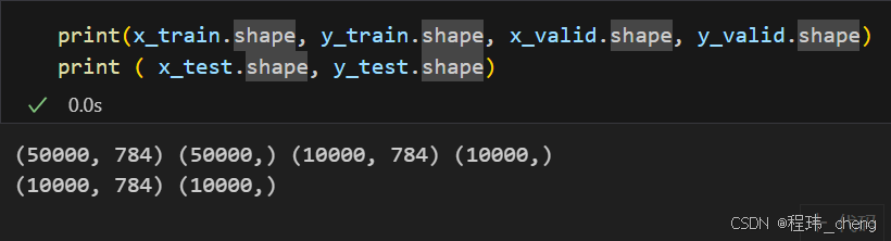
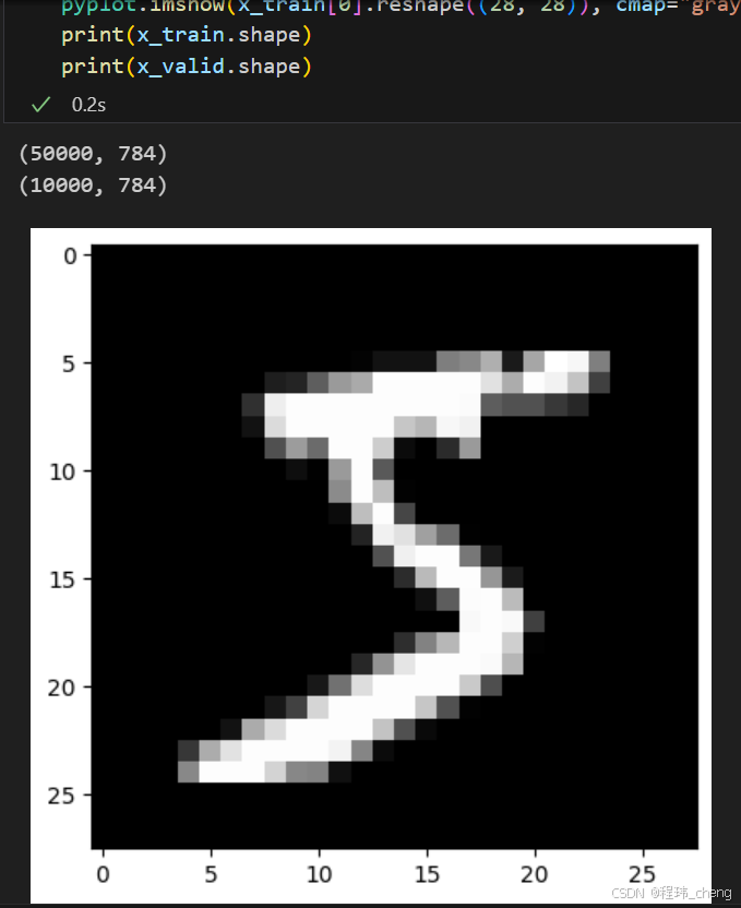
验证一下：显示 x_train 中的第一张图像，同时打印 x_train 的形状，以便了解数据的整体结构。

from matplotlib import pyplot
import numpy as np

# 显示 x_train 中的第一张图片
pyplot.imshow(x_train[0].reshape((28, 28)), cmap="gray")

# 打印 x_train 的形状
print(x_train.shape)

注:我们将原训练集(60,000 )划分为了训练集(50,000)与验证集(10,000)，最后才利用测试集进行模型的优度评价。

1.3其他下载方法

如果下载失败可进行如下的尝试：
(1)到官方网址下载：

https://pjreddie.com/projects/mnist-in-csv/ 

(2)利用pytorch下载：

参考：

[参考博客](https://blog.csdn.net/qq_41813454/article/details/136332315?ops_request_misc=%257B%2522request%255Fid%2522%253A%252279A92401-124C-40D4-9E56-C825EC4EF9B1%2522%252C%2522scm%2522%253A%252220140713.130102334..%2522%257D&request_id=79A92401-124C-40D4-9E56-C825EC4EF9B1&biz_id=0&utm_medium=distribute.pc_search_result.none-task-blog-2~all~baidu_landing_v2~default-4-136332315-null-null.142%5Ev100%5Epc_search_result_base9&utm_term=MNIST%E6%95%B0%E6%8D%AE%E9%9B%86%E7%9A%84%E4%B8%8B%E8%BD%BD&spm=1018.2226.3001.4187)

---

二、流程总览

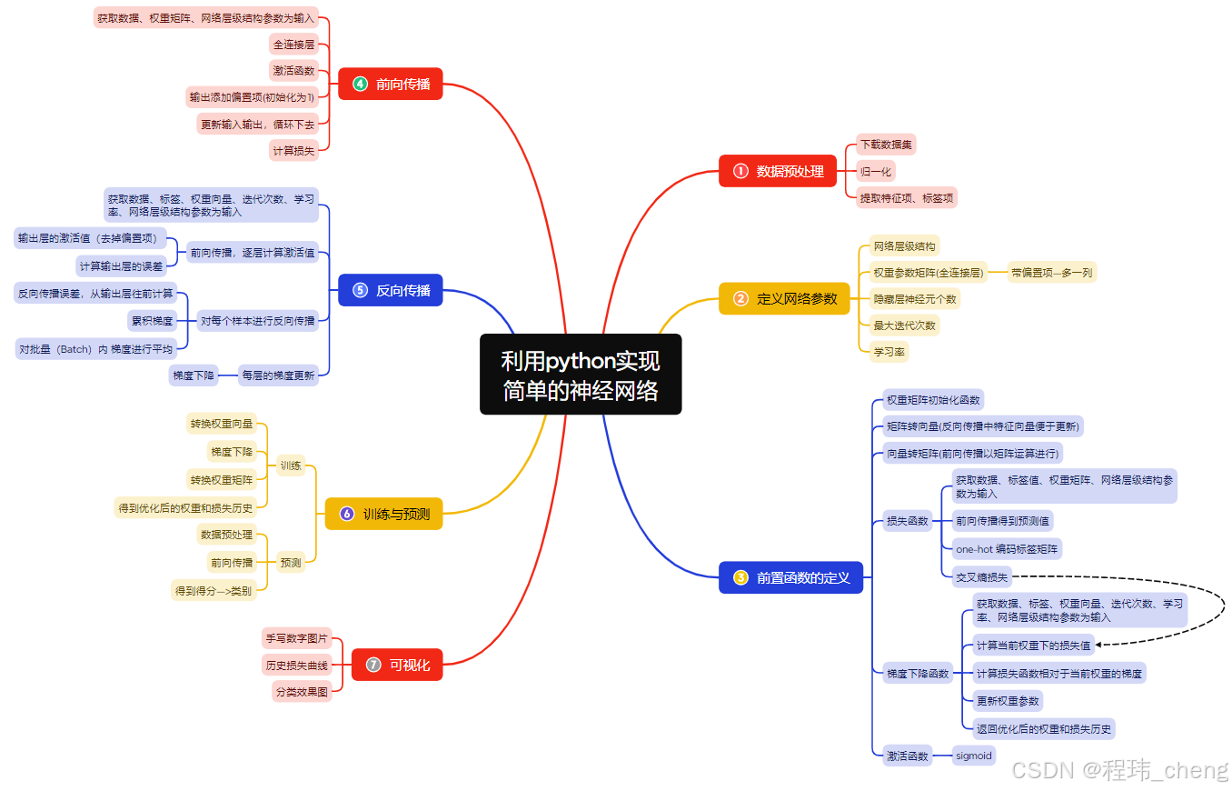
上图即此次实现神经网络的整体流程——首先，通过数据预处理获取和规范化输入数据，然后定义网络的层级结构、初始化权重参数，并设置学习率等超参数。在前向传播中，逐层计算激活值，并通过损失函数评估模型的预测误差。随后，利用反向传播计算各层的梯度，更新权重以优化模型。训练过程中，通过迭代使误差收敛，最终在测试集上进行预测。同时，通过可视化技术，如损失曲线和分类效果图，直观地评估和分析模型的性能。

下面则按照图片内容逐步实现，设计一个简单的神经网络。

---

先导入需要的库。

import numpy as np
import sys
sys.path.append('D:/360MoveData/Users/123/Desktop/数据分析/神经网络/utils')
from utils.features import prepare_for_training
from utils.hypothesis import sigmoid, sigmoid_gradient

三、构建网络的 MultilayerPerceptron 类

class MultilayerPerceptron:
    def __init__(self, data, labels, layers, normalize_data=False):
        """
        初始化函数

        参数:
        - data (numpy.ndarray): 输入数据。
        - labels (numpy.ndarray): 标签数据。
        - layers (list): 神经网络的层次结构列表。
        - normalize_data (bool): 指定是否对数据进行归一化处理。默认为 False。

        功能:
        - 调用数据预处理函数 prepare_for_training 对输入数据进行必要的预处理操作。
        - 根据需要对输入数据进行归一化处理。
        - 使用 thetas_init 函数初始化神经网络各层的权重矩阵。

        返回值:
        无（该方法为类的构造函数，不返回任何值）。
        """
        
        # 准备数据，并且调用了数据预处理函数 prepare_for_training
        data_processed = prepare_for_training(data, normalize_data=normalize_data)
        
        self.data = data_processed  # 处理后的数据
        self.labels = labels  # 标签数据
        self.layers = layers  # 神经网络的层结构
        self.normalize_data = normalize_data  # 是否归一化数据
        
        # 静态方法thetas_init 方法是一个专门用于初始化权重矩阵的函数.
        self.thetas = MultilayerPerceptron.thetas_init(layers)

四、 前置函数的定义

4.1权重矩阵初始化的 thetas_init 方法

    @staticmethod
    def thetas_init(layers):
        """
        初始化各层的权重参数矩阵。

        参数:
        - layers (list): 神经网络的层次结构列表。

        返回值:
        - thetas (dict): 包含每层到下一层的权重矩阵的字典。

        功能:
        - 遍历神经网络的每一层，除了最后一层，因为最后一层没有下一层。
        - 为每一层和下一层之间创建一个权重矩阵，形状为 [out_count, in_count + 1]。
        - 使用随机值初始化权重，并进行适当的缩放，避免梯度消失或爆炸。
        """
        num_layers = len(layers)
        
        thetas = {}
        
        # 遍历每一层，除了最后一层，因为最后一层没有下一层
        for layer_index in range(num_layers - 1):
            """
            遍历网络的每一层，生成各层的权重参数矩阵。
            例如，对于层结构 [784, 25, 10]：
            - 第一个循环将生成一个大小为 [25, 785] 的矩阵，表示从输入层到隐藏层的权重矩阵（包含偏置）。
            - 第二个循环将生成一个大小为 [10, 26] 的矩阵，表示从隐藏层到输出层的权重矩阵（包含偏置）。
            """
            in_count = layers[layer_index]
            out_count = layers[layer_index + 1]
            
            # 初始化权重矩阵，形状为 [out_count, in_count + 1]，+1 是因为包括了偏置项
            thetas[layer_index] = np.random.rand(out_count, in_count + 1) * 0.05
            # 使用 0.05 作为缩放因子，使得权重初始值较小，避免梯度消失或爆炸问题
        
        return thetas

4.2矩阵—>向量的 thetas_unroll 方法

    '''
       thetas_unroll 方法的作用是将神经网络中的权重矩阵展平（unroll）成一个一维数组。
    '''
    @staticmethod
    def thetas_unroll(thetas):
        num_theta_layers = len(thetas) 
        unrolled_theta = np.array([]) 
        for theta_layer_index in range(num_theta_layers):
            
            # 将每一层的权重矩阵展平为一维数组，并水平堆叠到 unrolled_theta 中
            unrolled_theta = np.hstack((unrolled_theta,thetas[theta_layer_index].flatten()))
            
        return unrolled_theta  # 返回展开后的权重向量

4.3向量—>矩阵的 thetas_roll 方法

    '''
        thetas_roll将原来展平的特征向量重新组装为权重矩阵
    '''
    @staticmethod       
    def thetas_roll(unrolled_thetas,layers):    
        num_layers = len(layers)
        thetas = {}
        unrolled_shift = 0  # 初始化指针，用于追踪一维数组中的位置
        
        for layer_index in range(num_layers - 1):
            in_count = layers[layer_index]
            out_count = layers[layer_index + 1]
    
            # 确定每个层权重矩阵的大小
            thetas_width = in_count + 1  # +1 是因为有偏置项
            thetas_height = out_count  
            thetas_volume = thetas_width * thetas_height
    
            # 从展平的权重向量中提取对应当前层的权重值
            start_index = unrolled_shift
            end_index = unrolled_shift + thetas_volume  
            layer_theta_unrolled = unrolled_thetas[start_index:end_index] 
    
            # 将展平的权重重构为原来的形状，即 [out_count, in_count + 1]
            thetas[layer_index] = layer_theta_unrolled.reshape((thetas_height, thetas_width))
            # 更新指针的位置，移动到下一个层的权重开始的位置
            unrolled_shift = unrolled_shift + thetas_volume
        
        return thetas 

4.4损失函数 cost_function

    @staticmethod        
    def cost_function(data, labels, thetas, layers):
        """
        计算损失函数

        参数:
        - data (numpy.ndarray): 输入数据矩阵。
        - labels (numpy.ndarray): 标签数据。
        - thetas (dict): 各层的权重参数字典。
        - layers (list): 神经网络的层次结构列表。

        返回值:
        - cost (float): 计算得到的交叉熵损失值。
        """
        
        num_layers = len(layers)  
        num_examples = data.shape[0]
        num_labels = layers[-1] 
        predictions = MultilayerPerceptron.feedforward_propagation(data, thetas, layers)
        
        # 创建 one-hot 编码标签矩阵
        bitwise_labels = np.zeros((num_examples, num_labels))
        for example_index in range(num_examples):
            # 将每个样本的实际标签转换为 one-hot 编码，位置为1，其它为0
            bitwise_labels[example_index][labels[example_index][0]] = 1
        
        # 计算损失值
        # bit_set_cost: 计算当真实标签为1时的预测损失，log函数用于计算交叉熵损失
        bit_set_cost = np.sum(np.log(predictions[bitwise_labels == 1]))
        # bit_not_set_cost: 计算当真实标签为0时的预测损失
        bit_not_set_cost = np.sum(np.log(1 - predictions[bitwise_labels == 0]))
        # 计算总的代价函数值：使用交叉熵损失函数的标准公式
        cost = (-1 / num_examples) * (bit_set_cost + bit_not_set_cost)
        
        return cost

4.5梯度计算函数 gradient_step

    @staticmethod 
    def gradient_step(data, labels, optimized_theta, layers):
        """
        计算当前权重下的梯度。
        
        参数：
        - data: 输入数据
        - labels: 真实标签
        - optimized_theta: 当前展开的权重参数
        - layers: 神经网络的层次结构
        
        返回值：
        - thetas_unrolled_gradients: 未展开的权重梯度，用于更新权重
        """
        
        # 将展开的权重转换回每层的权重矩阵形式
        theta = MultilayerPerceptron.thetas_roll(optimized_theta, layers)
    
        # 通过反向传播计算每层的权重梯度
        thetas_rolled_gradients = MultilayerPerceptron.back_propagation(data, labels, theta, layers)
    
        # 将计算得到的梯度展开为向量形式
        thetas_unrolled_gradients = MultilayerPerceptron.thetas_unroll(thetas_rolled_gradients)
        
        return thetas_unrolled_gradients  # 返回展开的权重梯度

4.6梯度下降函数 gradient_descent

    @staticmethod
    def gradient_descent(data, labels, unrolled_theta, layers, max_iterations, alpha):
        """
        使用梯度下降算法优化神经网络的权重参数。
        
        参数：
        - data: 输入数据
        - labels: 真实标签
        - unrolled_theta: 已展开的初始权重参数向量
        - layers: 神经网络的层次结构
        - max_iterations: 最大迭代次数
        - alpha: 学习率
        
        返回值：
        - optimized_theta: 经过优化后的权重参数
        - cost_history: 每次迭代的损失历史
        """
        
        optimized_theta = unrolled_theta  # 初始化权重参数
        cost_history = []  # 用于存储每次迭代的损失值
        
        # 进行 max_iterations 次梯度下降
        for _ in range(max_iterations): 
            # 1. 计算当前权重下的损失值
            cost = MultilayerPerceptron.cost_function(data, labels, MultilayerPerceptron.thetas_roll(optimized_theta, layers), layers)
            cost_history.append(cost)  # 记录损失值
    
            # 2. 计算损失函数相对于当前权重的梯度
            theta_gradient = MultilayerPerceptron.gradient_step(data, labels, optimized_theta, layers)
    
            # 3. 更新权重参数：optimized_theta = optimized_theta - alpha * 梯度
            optimized_theta = optimized_theta - alpha * theta_gradient
        
        return optimized_theta, cost_history  # 返回优化后的权重和损失历史

五、前向传播过程 feedforward_propagation

    @staticmethod        
    def feedforward_propagation(data, thetas, layers):  
        """
        前向传播

        参数:
        - data (numpy.ndarray): 输入数据矩阵。
        - thetas (dict): 各层的权重参数字典。
        - layers (list): 神经网络的层次结构列表。

        返回值:
        - in_layer_activation (numpy.ndarray): 最后一层的输出结果（不包含偏置项）。

        功能:
        - 在输入数据中显式添加偏置项，以确保在隐藏层和输出层的矩阵计算中维度匹配。
        - 逐层计算每一层的激活值，并在每层的输出中添加偏置项以传递到下一层。
        - 返回最终输出层的激活值，同时去除偏置项。
        """
        
        num_layers = len(layers)  
        num_examples = data.shape[0]  
        # 处理输入数据的维度，显式添加偏置项（即在第一列添加1）防止后续矩阵计算维度不匹配
        data = np.hstack((np.ones((data.shape[0], 1)), data))
        in_layer_activation = data  
        
        for layer_index in range(num_layers - 1):
            theta = thetas[layer_index]  
            # 计算当前层的输出: 激活值 = sigmoid(输入 * 权重(含偏置项))
            out_layer_activation = sigmoid(np.dot(in_layer_activation, theta.T))
            # 添加偏置项: 在输出激活值的第一列添加一列全为1的偏置项
            out_layer_activation = np.hstack((np.ones((num_examples, 1)), out_layer_activation))
            in_layer_activation = out_layer_activation
    
        # 返回输出层的激活值，去除偏置项（偏置项位于第一列，所以去除第一列）
        return in_layer_activation[:, 1:]

六、反向传播过程 back_propagation

    @staticmethod 
    def back_propagation(data, labels, thetas, layers):
        """
        实现神经网络的反向传播算法，计算每层的梯度。
        
        参数：
        - data: 输入数据，形状为 (num_examples, num_features)
        - labels: 真实标签，形状为 (num_examples, 1)
        - thetas: 神经网络各层的权重矩阵
        - layers: 神经网络的层次结构
        
        返回值：
        - deltas: 每层权重的梯度
        """
        
        num_layers = len(layers)  # 获取神经网络的层数

        # 处理输入数据的列数
        data = np.hstack((np.ones((data.shape[0], 1)), data))

        (num_examples, num_features) = data.shape  
        num_label_types = layers[-1] 
        deltas = {} 
        
        for layer_index in range(num_layers - 1):
            in_count = layers[layer_index]  
            out_count = layers[layer_index + 1]  
            # 每层的梯度矩阵初始化为 0，形状为 (输出神经元数, 输入神经元数 + 1)，+1 是因为偏置项
            deltas[layer_index] = np.zeros((out_count, in_count + 1))  
            
        # 对每个样本进行反向传播
        for example_index in range(num_examples):
            layers_inputs = {}  # 存储每层的输入（加权和）
            layers_activations = {}  # 存储每层的激活值
            layers_activation = data[example_index, :].reshape((num_features, 1))  # 获取当前样本的输入，并转置为列向量
            layers_activations[0] = layers_activation  # 输入层的激活值就是原始数据
            
            # 前向传播，逐层计算激活值
            for layer_index in range(num_layers - 1):
                layer_theta = thetas[layer_index]  # 获取当前层的权重矩阵
                layer_input = np.dot(layer_theta, layers_activation)  # 计算当前层的输入 (加权和)
                layers_activation = np.vstack((np.array([[1]]), sigmoid(layer_input)))  # 对输入应用激活函数，添加偏置
                layers_inputs[layer_index + 1] = layer_input  # 保存当前层的输入
                layers_activations[layer_index + 1] = layers_activation  # 保存当前层的激活值
            
            # 输出层的激活值（去掉偏置项）
            output_layer_activation = layers_activation[1:, :]
            
            delta = {}  # 存储每层的误差
            # 将标签转换为 one-hot 编码
            bitwise_label = np.zeros((num_label_types, 1))  # 初始化 one-hot 标签
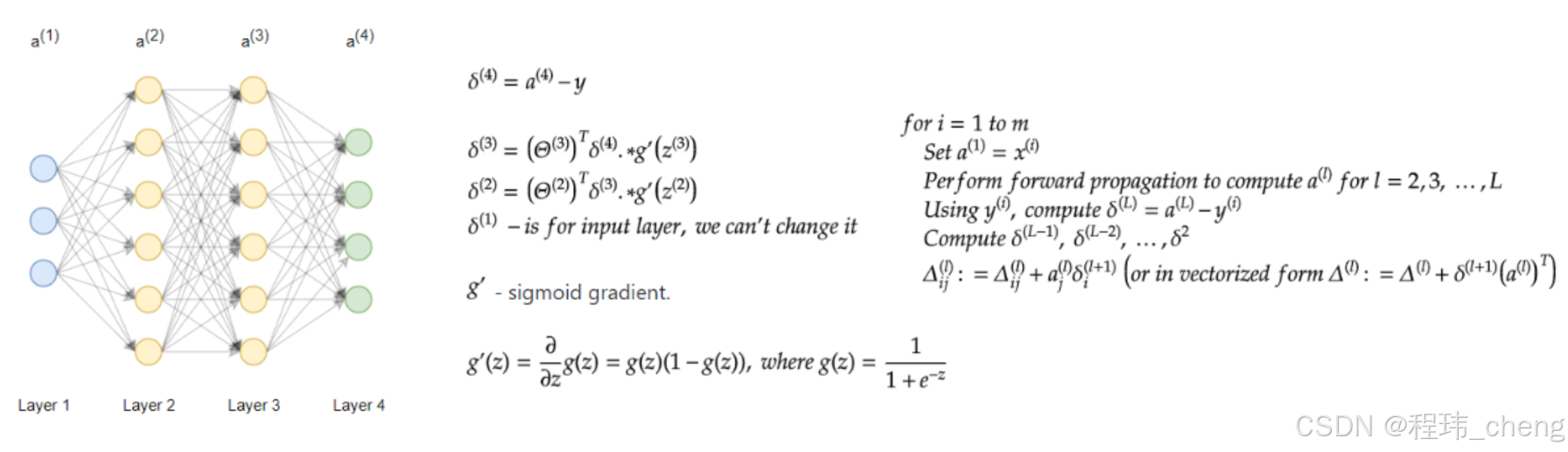
            bitwise_label[labels[example_index][0]] = 1  # 将正确的标签置为 1
            
            # 计算输出层的误差：delta_L = a_L - y
            delta[num_layers - 1] = output_layer_activation - bitwise_label
            
            # 反向传播误差，从输出层往前计算
            for layer_index in range(num_layers - 2, 0, -1):
                layer_theta = thetas[layer_index]  # 获取当前层的权重
                next_delta = delta[layer_index + 1]  # 获取下一层的误差
                layer_input = layers_inputs[layer_index]  # 获取当前层的输入
                layer_input = np.vstack((np.array((1)), layer_input))  # 添加偏置
                # 计算当前层的误差：delta_l = (theta_l)^T * delta_{l+1} .* sigmoid'(z_l)
                delta[layer_index] = np.dot(layer_theta.T, next_delta) * sigmoid_gradient(layer_input)
                delta[layer_index] = delta[layer_index][1:, :]  # 去掉偏置项的误差
            
            # 累积梯度
            for layer_index in range(num_layers - 1):
                layer_delta = np.dot(delta[layer_index + 1], layers_activations[layer_index].T)  # 计算每层的梯度
                deltas[layer_index] = deltas[layer_index] + layer_delta  # 累积每层的梯度
        
        # 对梯度进行平均
        for layer_index in range(num_layers - 1):
            deltas[layer_index] = deltas[layer_index] * (1 / num_examples)
        
        return deltas  # 返回每层的梯度

七、应用神经网络进行分类

7.1数据预处理

train_data = data.sample(frac=0.8)
test_data = data.drop(train_data.index)

train_data = train_data.values
test_data = test_data.values

num_training_examples = 5000

x_train = train_data[:num_training_examples, 1:]
y_train = train_data[:num_training_examples, [0]]

x_test = test_data[:, 1:]
y_test = test_data[:, [0]]

7.2模型的训练

# 设置多层感知机的层级结构，使用一个隐藏层
layers = [784, 25, 10] 
normalize_data = True
max_iterations = 800
alpha = 0.1

# 实例化并训练模型
multilayer_perceptron = MultilayerPerceptron(x_train, y_train, layers, normalize_data)
thetas, costs = multilayer_perceptron.train(max_iterations, alpha)

7.3模型的预测

# 对训练集和测试集进行预测
y_train_predictions = multilayer_perceptron.predict(x_train)
y_test_predictions = multilayer_perceptron.predict(x_test)

# 计算并打印准确率
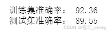
train_p = np.sum(y_train_predictions == y_train) / y_train.shape[0] * 100
test_p = np.sum(y_test_predictions == y_test) / y_test.shape[0] * 100
print('训练集准确率：', train_p)
print('测试集准确率：', test_p)

八、可视化展示

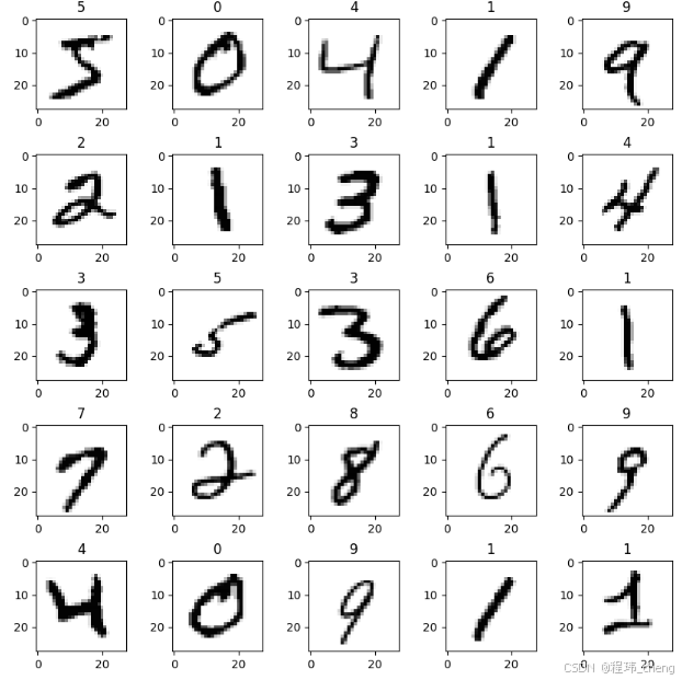
8.1数据可视化

data = pd.read_csv(r'./data/mnist-demo.csv')
numbers_to_display = 25
num_cells = math.ceil(math.sqrt(numbers_to_display))
plt.figure(figsize=(10,10))
for plot_index in range(numbers_to_display):
    digit = data[plot_index:plot_index+1].values
    digit_label = digit[0][0]
    digit_pixels = digit[0][1:]
    image_size = int(math.sqrt(digit_pixels.shape[0]))
    frame = digit_pixels.reshape((image_size, image_size))
    plt.subplot(num_cells, num_cells, plot_index + 1)
    plt.imshow(frame, cmap='Greys')
    plt.title(digit_label)
plt.subplots_adjust(wspace=0.5, hspace=0.5)
plt.show()

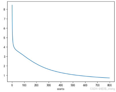
8.2损失曲线

# 绘制训练过程中损失的变化曲线
plt.plot(range(len(costs)), costs)
plt.xlabel('Gradient steps')
plt.ylabel('Costs')
plt.title('Training Loss Curve')
plt.show()

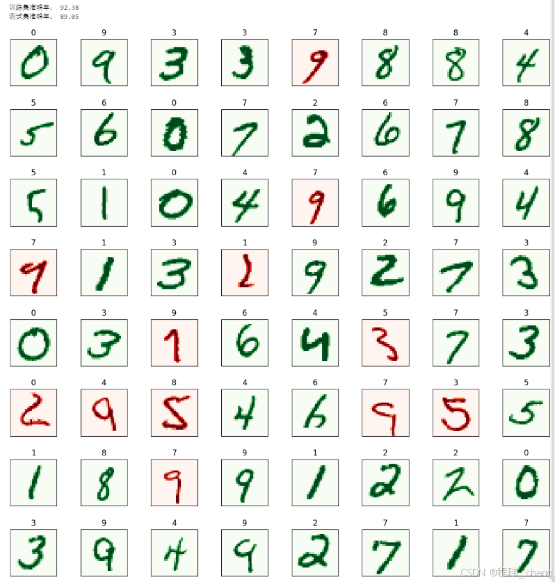
8.3分类效果图

# 设置要显示的测试图片数量
numbers_to_display = 64
num_cells = math.ceil(math.sqrt(numbers_to_display))
plt.figure(figsize=(15, 15))

for plot_index in range(numbers_to_display):
    digit_label = y_test[plot_index, 0]
    digit_pixels = x_test[plot_index, :]
    predicted_label = y_test_predictions[plot_index][0]

    image_size = int(math.sqrt(digit_pixels.shape[0]))
    frame = digit_pixels.reshape((image_size, image_size))

    # 预测正确显示为绿色，预测错误显示为红色
    color_map = 'Greens' if predicted_label == digit_label else 'Reds'
    plt.subplot(num_cells, num_cells, plot_index + 1)
    plt.imshow(frame, cmap=color_map)
    plt.title(predicted_label)
    plt.tick_params(axis='both', which='both', bottom=False, left=False, labelbottom=False, labelleft=False)

plt.subplots_adjust(hspace=0.5, wspace=0.5)
plt.show()

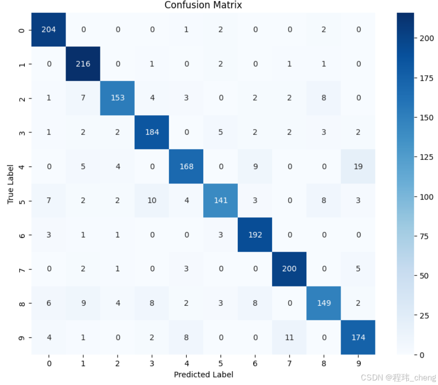
8.4混淆矩阵

from sklearn.metrics import confusion_matrix
import seaborn as sns

# 计算混淆矩阵
conf_matrix = confusion_matrix(y_test, y_test_predictions)

# 绘制混淆矩阵
plt.figure(figsize=(10, 8))
sns.heatmap(conf_matrix, annot=True, fmt='d', cmap='Blues')
plt.xlabel('Predicted Label')
plt.ylabel('True Label')
plt.title('Confusion Matrix')
plt.show()

---

完整代码

import numpy as np
from utils.features import prepare_for_training
from utils.hypothesis import sigmoid, sigmoid_gradient



class MultilayerPerceptron:
    def __init__(self,data,labels,layers,normalize_data =False):
        data_processed = prepare_for_training(data,normalize_data = normalize_data)[0]
        self.data= data_processed
        self.labels= labels
        self.layers= layers #784 25 10
        self.normalize_data= normalize_data
        self.thetas = MultilayerPerceptron.thetas_init(layers)
        
    def predict(self,data):
        data_processed = prepare_for_training(data,normalize_data = self.normalize_data)[0]
        num_examples = data_processed.shape[0]
        
        predictions = MultilayerPerceptron.feedforward_propagation(data_processed,self.thetas,self.layers)
        
        return np.argmax(predictions,axis=1).reshape((num_examples,1))
        
        
        
    def train(self,max_iterations=1000,alpha=0.1):
        unrolled_theta = MultilayerPerceptron.thetas_unroll(self.thetas)
        
        (optimized_theta,cost_history) = MultilayerPerceptron.gradient_descent(self.data,self.labels,unrolled_theta,self.layers,max_iterations,alpha)
        
        
        self.thetas = MultilayerPerceptron.thetas_roll(optimized_theta,self.layers)
        return self.thetas,cost_history
         
    @staticmethod
    def thetas_init(layers):
        num_layers = len(layers)
        thetas = {}
        for layer_index in range(num_layers - 1):
            """
                            会执行两次，得到两组参数矩阵：25*785 , 10*26
            """
            in_count = layers[layer_index]
            out_count = layers[layer_index+1]
            # 这里需要考虑到偏置项，记住一点偏置的个数跟输出的结果是一致的
            thetas[layer_index] = np.random.rand(out_count,in_count+1)*0.05 #随机进行初始化操作，值尽量小一点
        return thetas
    
    @staticmethod
    def thetas_unroll(thetas):
        num_theta_layers = len(thetas)
        unrolled_theta = np.array([])
        for theta_layer_index in range(num_theta_layers):
            unrolled_theta = np.hstack((unrolled_theta,thetas[theta_layer_index].flatten()))
        return unrolled_theta
    
    @staticmethod
    def gradient_descent(data,labels,unrolled_theta,layers,max_iterations,alpha):
        
        optimized_theta = unrolled_theta
        cost_history = []
        
        for _ in range(max_iterations):

            cost = MultilayerPerceptron.cost_function(data,labels,MultilayerPerceptron.thetas_roll(optimized_theta,layers),layers)
            cost_history.append(cost)
            theta_gradient = MultilayerPerceptron.gradient_step(data,labels,optimized_theta,layers)
            optimized_theta = optimized_theta - alpha* theta_gradient
        return optimized_theta,cost_history
            
            
    @staticmethod 
    def gradient_step(data,labels,optimized_theta,layers):
        theta = MultilayerPerceptron.thetas_roll(optimized_theta,layers)
        thetas_rolled_gradients = MultilayerPerceptron.back_propagation(data,labels,theta,layers)
        thetas_unrolled_gradients = MultilayerPerceptron.thetas_unroll(thetas_rolled_gradients)
        return thetas_unrolled_gradients
    
    @staticmethod 
    def back_propagation(data,labels,thetas,layers):
        num_layers = len(layers)
        (num_examples,num_features) = data.shape
        num_label_types = layers[-1]
        
        deltas = {}
        #初始化操作
        for layer_index in range(num_layers -1 ):
            in_count = layers[layer_index]
            out_count = layers[layer_index+1]
            deltas[layer_index] = np.zeros((out_count,in_count+1)) #25*785 10*26
        for example_index in range(num_examples):
            layers_inputs = {}
            layers_activations = {}
            layers_activation = data[example_index,:].reshape((num_features,1))#785*1
            layers_activations[0] = layers_activation
            #逐层计算
            for layer_index in range(num_layers - 1):
                layer_theta = thetas[layer_index] #得到当前权重参数值 25*785   10*26
                layer_input = np.dot(layer_theta,layers_activation) #第一次得到25*1 第二次10*1
                layers_activation = np.vstack((np.array([[1]]),sigmoid(layer_input)))
                layers_inputs[layer_index + 1] = layer_input #后一层计算结果
                layers_activations[layer_index + 1] = layers_activation #后一层经过激活函数后的结果
            output_layer_activation = layers_activation[1:,:]
            
            delta = {}
            #标签处理
            bitwise_label = np.zeros((num_label_types,1))
            bitwise_label[labels[example_index][0]] = 1
            #计算输出层和真实值之间的差异
            delta[num_layers - 1] = output_layer_activation - bitwise_label
            
            #遍历循环 L L-1 L-2 ...2
            for layer_index in range(num_layers - 2,0,-1):
                layer_theta = thetas[layer_index]
                next_delta = delta[layer_index+1]
                layer_input = layers_inputs[layer_index]
                layer_input = np.vstack((np.array((1)),layer_input))
                #按照公式进行计算
                delta[layer_index] = np.dot(layer_theta.T,next_delta)*sigmoid_gradient(layer_input)
                #过滤掉偏置参数
                delta[layer_index] = delta[layer_index][1:,:]
            for layer_index in range(num_layers-1):
                layer_delta = np.dot(delta[layer_index+1],layers_activations[layer_index].T)
                deltas[layer_index] = deltas[layer_index] + layer_delta #第一次25*785  第二次10*26
                
        for layer_index in range(num_layers -1):
               
            deltas[layer_index] = deltas[layer_index] * (1/num_examples)
            
        return deltas
            
    @staticmethod        
    def cost_function(data,labels,thetas,layers):
        num_layers = len(layers)
        num_examples = data.shape[0]
        num_labels = layers[-1]
        
        #前向传播走一次
        predictions = MultilayerPerceptron.feedforward_propagation(data,thetas,layers)
        #制作标签，每一个样本的标签都得是one-hot
        bitwise_labels = np.zeros((num_examples,num_labels))
        for example_index in range(num_examples):
            bitwise_labels[example_index][labels[example_index][0]] = 1
        bit_set_cost = np.sum(np.log(predictions[bitwise_labels == 1]))
        bit_not_set_cost = np.sum(np.log(1-predictions[bitwise_labels == 0]))
        cost = (-1/num_examples) *(bit_set_cost+bit_not_set_cost)
        return cost
                
    @staticmethod        
    def feedforward_propagation(data,thetas,layers):    
        num_layers = len(layers)
        num_examples = data.shape[0]
        in_layer_activation = data
        
        # 逐层计算
        for layer_index in range(num_layers - 1):
            theta = thetas[layer_index]
            out_layer_activation = sigmoid(np.dot(in_layer_activation,theta.T))
            # 正常计算完之后是num_examples25,但是要考虑偏置项 变成num_examples*26
            out_layer_activation = np.hstack((np.ones((num_examples,1)),out_layer_activation))
            in_layer_activation = out_layer_activation
            
        #返回输出层结果,结果中不要偏置项了
        return in_layer_activation[:,1:]
                   
    @staticmethod       
    def thetas_roll(unrolled_thetas,layers):    
        num_layers = len(layers)
        thetas = {}
        unrolled_shift = 0
        for layer_index in range(num_layers - 1):
            in_count = layers[layer_index]
            out_count = layers[layer_index+1]
            
            thetas_width = in_count + 1
            thetas_height = out_count
            thetas_volume = thetas_width * thetas_height
            start_index = unrolled_shift
            end_index = unrolled_shift + thetas_volume
            layer_theta_unrolled = unrolled_thetas[start_index:end_index]
            thetas[layer_index] = layer_theta_unrolled.reshape((thetas_height,thetas_width))
            unrolled_shift = unrolled_shift+thetas_volume
        
        return thetas
        
        
        
    import numpy as np
from utils.features import prepare_for_training
from utils.hypothesis import sigmoid, sigmoid_gradient



class MultilayerPerceptron:
    def __init__(self,data,labels,layers,normalize_data =False):
        data_processed = prepare_for_training(data,normalize_data = normalize_data)[0]
        self.data= data_processed
        self.labels= labels
        self.layers= layers #784 25 10
        self.normalize_data= normalize_data
        self.thetas = MultilayerPerceptron.thetas_init(layers)
        
    def predict(self,data):
        data_processed = prepare_for_training(data,normalize_data = self.normalize_data)[0]
        num_examples = data_processed.shape[0]
        
        predictions = MultilayerPerceptron.feedforward_propagation(data_processed,self.thetas,self.layers)
        
        return np.argmax(predictions,axis=1).reshape((num_examples,1))
        
        
        
    def train(self,max_iterations=1000,alpha=0.1):
        unrolled_theta = MultilayerPerceptron.thetas_unroll(self.thetas)
        
        (optimized_theta,cost_history) = MultilayerPerceptron.gradient_descent(self.data,self.labels,unrolled_theta,self.layers,max_iterations,alpha)
        
        
        self.thetas = MultilayerPerceptron.thetas_roll(optimized_theta,self.layers)
        return self.thetas,cost_history
         
    @staticmethod
    def thetas_init(layers):
        num_layers = len(layers)
        thetas = {}
        for layer_index in range(num_layers - 1):
            """
                            会执行两次，得到两组参数矩阵：25*785 , 10*26
            """
            in_count = layers[layer_index]
            out_count = layers[layer_index+1]
            # 这里需要考虑到偏置项，记住一点偏置的个数跟输出的结果是一致的
            thetas[layer_index] = np.random.rand(out_count,in_count+1)*0.05 #随机进行初始化操作，值尽量小一点
        return thetas
    
    @staticmethod
    def thetas_unroll(thetas):
        num_theta_layers = len(thetas)
        unrolled_theta = np.array([])
        for theta_layer_index in range(num_theta_layers):
            unrolled_theta = np.hstack((unrolled_theta,thetas[theta_layer_index].flatten()))
        return unrolled_theta
    
    @staticmethod
    def gradient_descent(data,labels,unrolled_theta,layers,max_iterations,alpha):
        
        optimized_theta = unrolled_theta
        cost_history = []
        
        for _ in range(max_iterations):

            cost = MultilayerPerceptron.cost_function(data,labels,MultilayerPerceptron.thetas_roll(optimized_theta,layers),layers)
            cost_history.append(cost)
            theta_gradient = MultilayerPerceptron.gradient_step(data,labels,optimized_theta,layers)
            optimized_theta = optimized_theta - alpha* theta_gradient
        return optimized_theta,cost_history
            
            
    @staticmethod 
    def gradient_step(data,labels,optimized_theta,layers):
        theta = MultilayerPerceptron.thetas_roll(optimized_theta,layers)
        thetas_rolled_gradients = MultilayerPerceptron.back_propagation(data,labels,theta,layers)
        thetas_unrolled_gradients = MultilayerPerceptron.thetas_unroll(thetas_rolled_gradients)
        return thetas_unrolled_gradients
    
    @staticmethod 
    def back_propagation(data,labels,thetas,layers):
        num_layers = len(layers)
        (num_examples,num_features) = data.shape
        num_label_types = layers[-1]
        
        deltas = {}
        #初始化操作
        for layer_index in range(num_layers -1 ):
            in_count = layers[layer_index]
            out_count = layers[layer_index+1]
            deltas[layer_index] = np.zeros((out_count,in_count+1)) #25*785 10*26
        for example_index in range(num_examples):
            layers_inputs = {}
            layers_activations = {}
            layers_activation = data[example_index,:].reshape((num_features,1))#785*1
            layers_activations[0] = layers_activation
            #逐层计算
            for layer_index in range(num_layers - 1):
                layer_theta = thetas[layer_index] #得到当前权重参数值 25*785   10*26
                layer_input = np.dot(layer_theta,layers_activation) #第一次得到25*1 第二次10*1
                layers_activation = np.vstack((np.array([[1]]),sigmoid(layer_input)))
                layers_inputs[layer_index + 1] = layer_input #后一层计算结果
                layers_activations[layer_index + 1] = layers_activation #后一层经过激活函数后的结果
            output_layer_activation = layers_activation[1:,:]
            
            delta = {}
            #标签处理
            bitwise_label = np.zeros((num_label_types,1))
            bitwise_label[labels[example_index][0]] = 1
            #计算输出层和真实值之间的差异
            delta[num_layers - 1] = output_layer_activation - bitwise_label
            
            #遍历循环 L L-1 L-2 ...2
            for layer_index in range(num_layers - 2,0,-1):
                layer_theta = thetas[layer_index]
                next_delta = delta[layer_index+1]
                layer_input = layers_inputs[layer_index]
                layer_input = np.vstack((np.array((1)),layer_input))
                #按照公式进行计算
                delta[layer_index] = np.dot(layer_theta.T,next_delta)*sigmoid_gradient(layer_input)
                #过滤掉偏置参数
                delta[layer_index] = delta[layer_index][1:,:]
            for layer_index in range(num_layers-1):
                layer_delta = np.dot(delta[layer_index+1],layers_activations[layer_index].T)
                deltas[layer_index] = deltas[layer_index] + layer_delta #第一次25*785  第二次10*26
                
        for layer_index in range(num_layers -1):
               
            deltas[layer_index] = deltas[layer_index] * (1/num_examples)
            
        return deltas
            
    @staticmethod        
    def cost_function(data,labels,thetas,layers):
        num_layers = len(layers)
        num_examples = data.shape[0]
        num_labels = layers[-1]
        
        #前向传播走一次
        predictions = MultilayerPerceptron.feedforward_propagation(data,thetas,layers)
        #制作标签，每一个样本的标签都得是one-hot
        bitwise_labels = np.zeros((num_examples,num_labels))
        for example_index in range(num_examples):
            bitwise_labels[example_index][labels[example_index][0]] = 1
        bit_set_cost = np.sum(np.log(predictions[bitwise_labels == 1]))
        bit_not_set_cost = np.sum(np.log(1-predictions[bitwise_labels == 0]))
        cost = (-1/num_examples) *(bit_set_cost+bit_not_set_cost)
        return cost
                
    @staticmethod        
    def feedforward_propagation(data,thetas,layers):    
        num_layers = len(layers)
        num_examples = data.shape[0]
        in_layer_activation = data
        
        # 逐层计算
        for layer_index in range(num_layers - 1):
            theta = thetas[layer_index]
            out_layer_activation = sigmoid(np.dot(in_layer_activation,theta.T))
            # 正常计算完之后是num_examples25,但是要考虑偏置项 变成num_examples*26
            out_layer_activation = np.hstack((np.ones((num_examples,1)),out_layer_activation))
            in_layer_activation = out_layer_activation
            
        #返回输出层结果,结果中不要偏置项了
        return in_layer_activation[:,1:]
                   
    @staticmethod       
    def thetas_roll(unrolled_thetas,layers):    
        num_layers = len(layers)
        thetas = {}
        unrolled_shift = 0
        for layer_index in range(num_layers - 1):
            in_count = layers[layer_index]
            out_count = layers[layer_index+1]
            
            thetas_width = in_count + 1
            thetas_height = out_count
            thetas_volume = thetas_width * thetas_height
            start_index = unrolled_shift
            end_index = unrolled_shift + thetas_volume
            layer_theta_unrolled = unrolled_thetas[start_index:end_index]
            thetas[layer_index] = layer_theta_unrolled.reshape((thetas_height,thetas_width))
            unrolled_shift = unrolled_shift+thetas_volume
        
        return thetas

import numpy as np
import pandas as pd
import matplotlib.pyplot as plt
import matplotlib.image as mping 
import math

from multilayer_perceptron import MultilayerPerceptron


data = pd.read_csv('../data/mnist-demo.csv')
numbers_to_display = 25
num_cells = math.ceil(math.sqrt(numbers_to_display))
plt.figure(figsize=(10,10))
for plot_index in range(numbers_to_display):
    digit = data[plot_index:plot_index+1].values
    digit_label = digit[0][0]
    digit_pixels = digit[0][1:]
    image_size = int(math.sqrt(digit_pixels.shape[0]))
    frame = digit_pixels.reshape((image_size,image_size))
    plt.subplot(num_cells,num_cells,plot_index+1)
    plt.imshow(frame,cmap='Greys')
    plt.title(digit_label)
plt.subplots_adjust(wspace=0.5,hspace=0.5)
plt.show()

train_data = data.sample(frac = 0.8)
test_data = data.drop(train_data.index)

train_data = train_data.values
test_data = test_data.values

num_training_examples = 5000

x_train = train_data[:num_training_examples,1:]
y_train = train_data[:num_training_examples,[0]]

x_test = test_data[:,1:]
y_test = test_data[:,[0]]


layers=[784,25,10]

normalize_data = True
max_iterations = 500
alpha = 0.1


multilayer_perceptron = MultilayerPerceptron(x_train,y_train,layers,normalize_data)
(thetas,costs) = multilayer_perceptron.train(max_iterations,alpha)
plt.plot(range(len(costs)),costs)
plt.xlabel('Grident steps')
plt.xlabel('costs')
plt.show()


y_train_predictions = multilayer_perceptron.predict(x_train)
y_test_predictions = multilayer_perceptron.predict(x_test)

train_p = np.sum(y_train_predictions == y_train)/y_train.shape[0] * 100
test_p = np.sum(y_test_predictions == y_test)/y_test.shape[0] * 100
print ('训练集准确率：',train_p)
print ('测试集准确率：',test_p)

numbers_to_display = 64

num_cells = math.ceil(math.sqrt(numbers_to_display))

plt.figure(figsize=(15, 15))

for plot_index in range(numbers_to_display):
    digit_label = y_test[plot_index, 0]
    digit_pixels = x_test[plot_index, :]
    
    predicted_label = y_test_predictions[plot_index][0]

    image_size = int(math.sqrt(digit_pixels.shape[0]))
    
    frame = digit_pixels.reshape((image_size, image_size))
    
    color_map = 'Greens' if predicted_label == digit_label else 'Reds'
    plt.subplot(num_cells, num_cells, plot_index + 1)
    plt.imshow(frame, cmap=color_map)
    plt.title(predicted_label)
    plt.tick_params(axis='both', which='both', bottom=False, left=False, labelbottom=False, labelleft=False)

plt.subplots_adjust(hspace=0.5, wspace=0.5)
plt.show()

总结

通过以上步骤，我们使用 Python 从零实现了一个基础的多层感知机神经网络，针对 MNIST 数据集进行了完整的训练和预测流程。在此过程中，我们从数据的预处理入手，设计了前向传播、反向传播、损失计算、梯度下降等核心函数。通过多次迭代训练，模型在测试集上达到了较好的识别效果。最后，我们利用数据可视化进一步分析了训练过程和模型表现，加深了对 BP 神经网络内部运作机制的理解。

本流程展示了如何逐步构建和训练一个神经网络的全过程，为进一步探索更深层的神经网络、卷积神经网络等奠定了基础。当然在实际情况下不需要我们这样实现各个函数，直接利用pytorch、TensorFlow或者Keras即可，后续就来说说pytorch框架的学习。