模拟退火算法实现TSP问题最优解
模拟退火算法通过模拟这一过程,允许暂时接受较差的解,以避免陷入局部最优,从而更有可能找到全局最优解。- 若 ( Delta E ≥ 0 \)(更差),以概率 P=e的(-Delta E/T)冷却率(`cooling_rate=0.995`):降温速度过快,全局搜索时间不足。迭代次数(`iterations=10000`):对于48城市问题,迭代次数不足。初始温度(`temp=1000`):可能过低
1. 灵感来源:冶金退火
在冶金中,退火是先将金属加热至高温,再缓慢冷却的过程。高温时原子活跃,逐渐降温时原子趋于有序,最终形成低能态的稳定结构。
模拟退火算法通过模拟这一过程,允许暂时接受较差的解(高温),以避免陷入局部最优,从而更有可能找到全局最优解。
---
2. 核心思想
温度参数(T ):控制搜索的“激进程度”。
高温时:算法接受较差解的概率较高,倾向于全局探索。
低温时:主要接受更优解,倾向于局部精细搜索。
降温策略:温度按一定速率(如指数衰减)逐步降低,最终趋近于零。
---
3. 算法步骤
1. 初始化
生成初始解(如随机路径)。
- 设定初始温度 ( T initial)、终止温度 ( T_final)、降温速率 a。
2. 迭代搜索
生成邻域解:通过微小扰动(如交换两个城市)生成新解。
计算能量差:比较新解与当前解的目标函数值差(如路径总距离变化量 ( Delta E )。
Metropolis准则:决定是否接受新解:
- 若 ( Delta E < 0 )(更优),直接接受。
- 若 ( Delta E ≥ 0 \)(更差),以概率 P=e的(-Delta E/T)
3. **降温**
- 更新温度:( T = a*T )。
- 重复迭代,直到终止条件
import numpy as np
import matplotlib.pyplot as plt

# 加载48个城市的坐标数据(补全的节点数据)
nodes = [
    (6734, 1453), (2233, 10), (5530, 1424), (401, 841),
    (3082, 1644), (7608, 4458), (7573, 3716), (7265, 1268),
    (6898, 1885), (1112, 2049), (5468, 2606), (5989, 2873),
    (4706, 2674), (4612, 2035), (6347, 2683), (6107, 669),
    (7611, 5184), (7462, 3590), (7732, 4723), (5900, 3561),
    (4483, 3369), (6101, 1110), (5199, 2182), (1633, 2809),
    (4307, 2322), (675, 1006), (7555, 4819), (7541, 3981),
    (3177, 756), (7352, 4506), (7545, 2801), (3245, 3305),
    (6426, 3173), (4608, 1198), (23, 2216), (7248, 3779),
    (7762, 4595), (7392, 2244), (3484, 2829), (6271, 2135),
    (4985, 140), (1916, 1569), (7280, 4899), (7509, 3239),
    (10, 2676), (6807, 2993), (5185, 3258), (3023, 1942)
]

def distance_matrix(coords):
    n = len(coords)
    dist = np.zeros((n, n))//使用矩阵给存储
    for i in range(n):
        for j in range(n):
            dx = coords[i][0] - coords[j][0]
            dy = coords[i][1] - coords[j][1]
            dist[i][j] = np.sqrt(dx**2 + dy**2)
    return dist
//计算两点的距离

def total_distance(path, dist):
    return sum(dist[path[i], path[i+1]] for i in range(len(path)-1)) + dist[path[-1], path[0]]
//计算总路径

def simulated_annealing(coords, iterations=10000, temp=1000, cooling_rate=0.995):
    dist = distance_matrix(coords)
    n = len(coords)
    current_path = list(range(n))//列出从第一个节点到第四十八个
    np.random.shuffle(current_path)//使用 NumPy 库中的 shuffle 函数对列表 current_path 进行原地(in-place)随机打乱操作。
    current_cost = total_distance(current_path, dist)//计算当前顺序的总路径

    best_path = current_path.copy()
    best_cost = current_cost

    for _ in range(iterations):
        temp *= cooling_rate//通过乘于冷却力,降低温度,实现对最坏结果减少接受
        # 生成新路径:随机交换两个城市
        new_path = current_path.copy()
        i, j = np.random.choice(n, 2, replace=False)//交换路径
        new_path[i], new_path[j] = new_path[j], new_path[i]
        new_cost = total_distance(new_path, dist)

        if new_cost < current_cost or np.random.rand() < np.exp((current_cost - new_cost)/temp):
            current_path = new_path
            current_cost = new_cost
            //如果新的路径成本比当前路径的成本低,或者满足Metropolis准则(即接受概率exp((current_cost - new_cost) / temp)大于一个介于0和1之间的随机数),则接受新路径作为当前路径,并更新当前成本current_cost。
            if current_cost < best_cost:
                best_path = current_path.copy()
                best_cost = current_cost

    return best_path, best_cost

# 计算最优路径
best_path, best_cost = simulated_annealing(nodes)
print("Optimal Path:", best_path)
print("Total Distance:", best_cost)

# 绘制路线图
plt.figure(figsize=(12, 8))
x = [nodes[i][0] for i in best_path]
y = [nodes[i][1] for i in best_path]
x.append(x[0])  # 闭合路径
y.append(y[0])

plt.plot(x, y, 'o-', markersize=5)
plt.title('Optimal TSP Route for att48')
plt.xlabel('Longitude')
plt.ylabel('Latitude')
plt.grid(True)
plt.show()
最终实现的效果

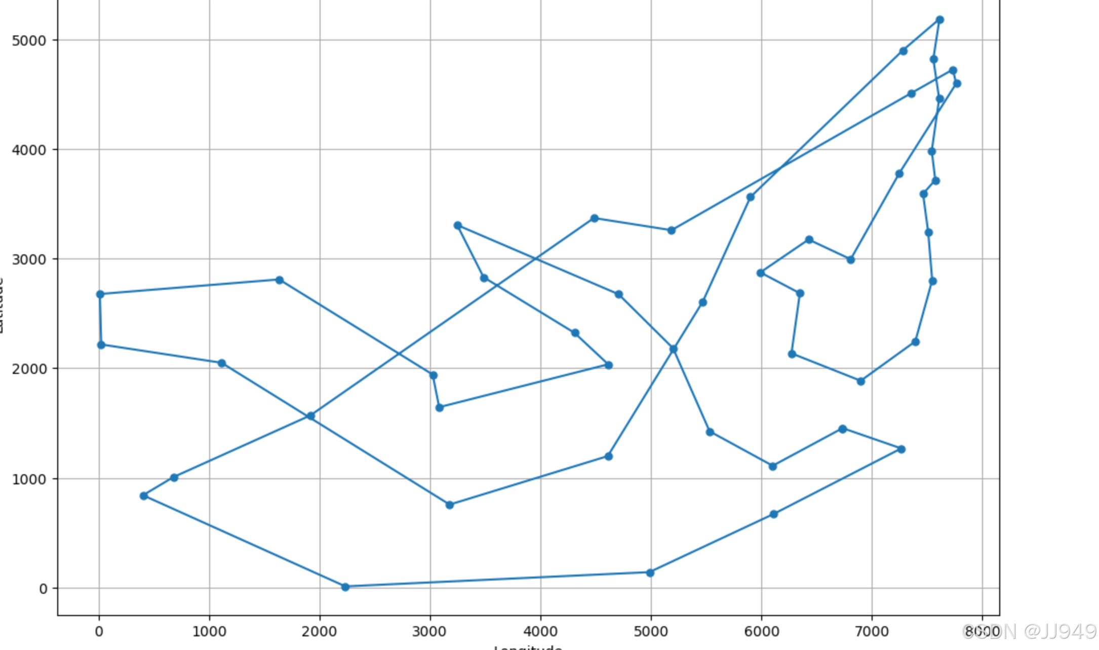
但是可以看出代码实现的结果并不理想,可能的原因是因为
1. 参数调优
问题分析
初始温度(`temp=1000`):可能过低,导致早期无法充分探索解空间。
迭代次数(`iterations=10000`):对于48城市问题,迭代次数不足。
冷却率(`cooling_rate=0.995`):降温速度过快,全局搜索时间不足。
如何改进
优化建议
提高初始温度(如 `temp=1e5`),确保高温阶段能接受更多差解。
增加迭代次数(如 `iterations=1e5`),延长搜索时间。
降低冷却率(如 `cooling_rate=0.999`),减缓温度下降速度。

有“AI”的1024 = 2048,欢迎大家加入2048 AI社区
更多推荐


 2
2 0
0- 0


 已为社区贡献1条内容

所有评论(0)