一、数据

     样例：

[7.847052, 7.847052, 7.861221, 7.861221, 7.879992, 7.879992, 7.876299, 7.876299, 7.878486, 7.878486, 7.900652, 7.900652, 7.903645, 7.903645, 7.854282, 7.854282, 7.865836, 7.865836, 7.85722, 7.85722, 7.876628, 7.876628, 7.877401, 7.877401, 7.872376, 7.872376, 7.882677, 7.882677, 7.9303, 7.9303, 7.873454, 7.873454, 7.847972, 7.847972, 7.857702, 7.857702, 7.863321, 7.863321, 7.913106, 7.913106, 7.854888, 7.854888, 7.88435, 7.88435, 7.846352, 7.846352, 7.880454, 7.880454, 7.866756, 7.866756, 7.834005, 7.834005, 7.846012, 7.846012, 7.858556, 7.858556, 7.86018, 7.86018, 7.850832, 7.850832, 7.877022, 7.877022, 7.92092, 7.92092, 7.852294, 7.852294, 7.85357, 7.85357, 7.818242, 7.818242, 7.881651, 7.881651, 7.850259, 7.850259, 7.783525, 7.783525, 7.856933, 7.856933, 7.91781, 7.91781, 7.834368, 7.834368, 7.817041, 7.817041, 7.898605, 7.898605, 7.811373, 7.811373, 7.828355, 7.828355, 7.856659, 7.856659, 7.814879, 7.814879, 7.808907, 7.808907, 7.791056, 7.791056, 7.837157, 7.837157, 7.826362, 7.826362, 7.823533, 7.823533, 7.817393, 7.817393, 7.79637, 7.79637, 7.841807, 7.841807, 7.822591, 7.822591, 7.828559, 7.828559, 7.78874, 7.78874, 7.749334, 7.749334, 7.786999, 7.786999, 7.791524, 7.791524, 7.799031, 7.799031, 7.765405, 7.765405, 7.80096, 7.80096, 7.827931, 7.827931, 7.733088, 7.733088, 7.787344, 7.787344, 7.755536, 7.755536, 7.758845, 7.758845, 7.749628, 7.749628, 7.779116, 7.779116, 7.832106, 7.832106, 7.775674, 7.775674, 7.771487, 7.771487, 7.771093, 7.771093, 7.767197, 7.767197, 7.757173, 7.757173, 7.722776, 7.722776, 7.734206, 7.734206, 7.684559, 7.684559, 7.775128, 7.775128, 7.737986, 7.737986, 7.701965, 7.701965, 7.715754, 7.715754, 7.710277, 7.710277, 7.667412, 7.667412, 7.742961, 7.742961, 7.70308, 7.70308, 7.712651, 7.712651, 7.731994, 7.731994, 7.691126, 7.691126, 7.652417, 7.652417, 7.746188, 7.746188, 7.665182, 7.665182, 7.689594, 7.689594, 7.677002, 7.677002, 7.64691, 7.64691, 7.682892, 7.682892, 7.644273, 7.644273, 7.671918, 7.671918, 7.638771, 7.638771, 7.655274, 7.655274, 7.620933, 7.620933, 7.625898, 7.625898, 7.608748, 7.608748, 7.648459, 7.648459, 7.6179, 7.6179, 7.61589, 7.61589, 7.624984, 7.624984, 7.6265, 7.6265, 7.597749, 7.597749, 7.609596, 7.609596, 7.607451, 7.607451, 7.577724, 7.577724, 7.598199, 7.598199, 7.575906, 7.575906, 7.583542, 7.583542, 7.60148, 7.60148, 7.578442, 7.578442, 7.574488, 7.574488, 7.594924, 7.594924, 7.591222, 7.591222, 7.604303, 7.604303, 7.559752, 7.559752, 7.569139, 7.569139, 7.589339, 7.589339, 7.585811, 7.585811, 7.531218, 7.531218, 7.547246, 7.547246, 7.553769, 7.553769, 7.573433, 7.573433, 7.548723, 7.548723, 7.55005, 7.55005, 7.531356, 7.531356, 7.542047, 7.542047, 7.569587, 7.569587, 7.553211, 7.553211, 7.533874, 7.533874, 7.546453, 7.546453, 7.568928, 7.568928, 7.534145, 7.534145, 7.526124, 7.526124, 7.607778, 7.607778, 7.558777, 7.558777, 7.572871, 7.572871, 7.534176, 7.534176, 7.587736, 7.587736, 7.568015, 7.568015, 7.59178, 7.59178, 7.586547, 7.586547, 7.531622, 7.531622, 7.515041, 7.515041, 7.591128, 7.591128, 7.54633, 7.54633, 7.583436, 7.583436, 7.593883, 7.593883, 7.528608, 7.528608, 7.554562, 7.554562, 7.556822, 7.556822, 7.548283, 7.548283, 7.539525, 7.539525, 7.542031, 7.542031, 7.539231, 7.539231, 7.559134, 7.559134, 7.605355, 7.605355, 7.615304, 7.615304, 7.568856, 7.568856, 7.541826, 7.541826, 7.552145, 7.552145, 7.6066, 7.6066, 7.569725, 7.569725, 7.610045, 7.610045, 7.5634, 7.5634, 7.583215, 7.583215, 7.5574, 7.5574, 7.576777, 7.576777, 7.563014, 7.563014, 7.593048, 7.593048, 7.54597, 7.54597, 7.593953, 7.593953, 7.546234, 7.546234, 7.604224, 7.604224, 7.573527, 7.573527, 7.545564, 7.545564, 7.596433, 7.596433, 7.623194, 7.623194, 7.588892, 7.588892, 7.593085, 7.593085, 7.585039, 7.585039, 7.562752, 7.562752, 7.653739, 7.653739, 7.624229, 7.624229, 7.581889, 7.581889, 7.59096, 7.59096, 7.602383, 7.602383, 7.598147, 7.598147, 7.616537, 7.616537, 7.588967, 7.588967, 7.6227, 7.6227, 7.59414, 7.59414, 7.634737, 7.634737, 7.650053, 7.650053, 7.601601, 7.601601, 7.607094, 7.607094, 7.604154, 7.604154, 7.653798, 7.653798, 7.637756, 7.637756, 7.635662, 7.635662, 7.591595, 7.591595, 7.629102, 7.629102, 7.602751, 7.602751, 7.664392, 7.664392, 7.634714, 7.634714, 7.640305, 7.640305, 7.633754, 7.633754, 7.634167, 7.634167, 7.671303, 7.671303, 7.670649, 7.670649, 7.63429, 7.63429, 7.647388, 7.647388, 7.662635, 7.662635, 7.664729, 7.664729, 7.687655, 7.687655, 7.675528, 7.675528, 7.670189, 7.670189, 7.66714, 7.66714, 7.676405, 7.676405, 7.666862, 7.666862, 7.687397, 7.687397, 7.687032, 7.687032, 7.642547, 7.642547, 7.658711, 7.658711, 7.648631, 7.648631, 7.681562, 7.681562, 7.696832, 7.696832, 7.64584, 7.64584, 7.704039, 7.704039, 7.68247, 7.68247, 7.681534, 7.681534, 7.679872, 7.679872, 7.657672, 7.657672, 7.658507, 7.658507, 7.676341, 7.676341, 7.653059, 7.653059, 7.720812, 7.720812, 7.651661, 7.651661, 7.694259, 7.694259, 7.701054, 7.701054, 7.703844, 7.703844, 7.678211, 7.678211, 7.696155, 7.696155, 7.71259, 7.71259, 7.703784, 7.703784, 7.641358, 7.641358, 7.689364, 7.689364, 7.717315, 7.717315, 7.727433, 7.727433, 7.679932, 7.679932, 7.734458, 7.734458, 7.704147, 7.704147, 7.684818, 7.684818, 7.68562, 7.68562, 7.712635, 7.712635, 7.714056, 7.714056, 7.719432, 7.719432, 7.722846, 7.722846, 7.720745, 7.720745, 7.742729, 7.742729, 7.720476, 7.720476, 7.730032, 7.730032, 7.752233, 7.752233, 7.72582, 7.72582, 7.709961, 7.709961, 7.729821, 7.729821, 7.682561, 7.682561, 7.768028, 7.768028, 7.702901, 7.702901, 7.789418, 7.789418, 7.78648, 7.78648, 7.735015, 7.735015, 7.74724, 7.74724, 7.737715, 7.737715, 7.75681, 7.75681, 7.671495, 7.671495, 7.75067, 7.75067, 7.753993, 7.753993, 7.690138, 7.690138, 7.773944, 7.773944, 7.725274, 7.725274, 7.744515, 7.744515, 7.780931, 7.780931, 7.71099, 7.71099, 7.773583, 7.773583, 7.727797, 7.727797, 7.737937, 7.737937, 7.769005, 7.769005, 7.766638, 7.766638, 7.741453, 7.741453, 7.748314, 7.748314, 7.745565, 7.745565, 7.774443, 7.774443]

二、代码

# -*- coding: utf-8 -*-

import os
import numpy
from numpy import *
from pylab import *
import warnings
warnings.filterwarnings("ignore")

datapath = "C:/Users/tangqing/Desktop/saveDataList.txt"
savepicturenum = 0
savepicturepath = "./picture/"


#图片存储路径创建
isExists=os.path.exists(savepicturepath)
if not isExists:
    os.makedirs(savepicturepath)

def smooth(x,window_len=100,window='hanning'):
    s=numpy.r_[x[window_len-1:0:-1],x,x[-2:-window_len-1:-1]]#np.r_ 是将一系列的序列合并到一个数组中
    w=eval('numpy.'+window+'(window_len)')
    y=numpy.convolve(w/w.sum(),s,mode='valid')
    return y


def processingdata(linedata):
    #处理数据
    data_list = []
    linedata = linedata.strip('\n')
    linedata = linedata.strip('[')
    linedata = linedata.strip(']')
    num = list(map(float,linedata.split(",")))
    datalist = np.array(num)
    return datalist
    

def drawCurveWindows(x,windows,ws):
    #绘制原始曲线
    plot(x)
    #plot(ones(ws))
    for w in windows[1:]:
        eval('plot('+w+'(ws) )')#返回传入字符串的表达式的结果。

    axis([0,len(x),min(x),max(x)])#坐标轴行是0-30，列是0-1.1
    legend(windows)#图例
    title("Original curve windows")
    show()


def drawAWholeCurve(x,windows,savenum,savepath):
    #绘制一整条平滑曲线
    plot(x)
    for w in windows:
        plot(smooth(x,int(len(x)/10)+1,w))
    l=['original curve']
    l.extend(windows)
    legend(l)
    title("Smoothing Curve")
    plt.savefig(str(savepath)+str(savenum)+".jpg")
    #plt.show()
    plt.close()

def main(savenum):
    f = open(datapath)
    line = f.readline()
    while line:
        windowsList=['hanning', 'hamming', 'bartlett', 'blackman']
        xRaw = processingdata(line)
        #windowlength=len(line)
        y=smooth(xRaw)
        hold(True)#曲线叠加
        #drawCurveWindows(xRaw,windowsList,ws)
        drawAWholeCurve(xRaw,windowsList,savenum,savepicturepath)
        savenum += 1
        line = f.readline()
    f.colse()
    

if __name__=='__main__':
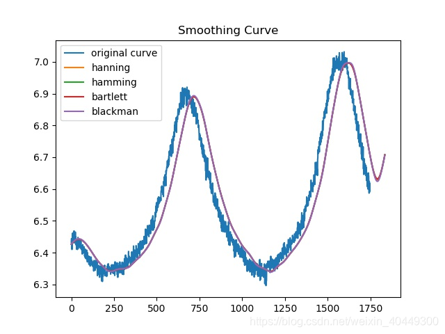
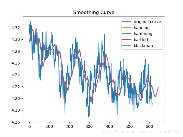
    main(savepicturenum)

三、平滑效果

四、预测

# -*- coding: utf-8 -*-
import os
import numpy
import matplotlib
#matplotlib.use('Agg')
import matplotlib.pyplot as plt
from pylab import *
from pandas import read_csv
import math
from keras.models import Sequential
from keras.layers import Dense
from keras.layers import LSTM
from sklearn.preprocessing import MinMaxScaler
from sklearn.metrics import mean_squared_error
from collections import OrderedDict
import pandas as pd

import warnings
warnings.filterwarnings("ignore")

datapath = "./data/DataList.txt"
savepicturenum = 0
savepicturepath = "./picture/"


#图片存储路径创建
isExists=os.path.exists(savepicturepath)
if not isExists:
    os.makedirs(savepicturepath)

#处理数据
def processingdata(linedata):
    print("Loading data ...")
    data_list = []
    linedata = linedata.strip('\n')
    linedata = linedata.strip('[')
    linedata = linedata.strip(']')
    num = list(map(float,linedata.split(",")))
    datalist = np.array(num)
    jd = range(len(datalist))
    return jd,datalist

#平滑函数
def smooth(x,window_len=200,window='hanning'):
    s=numpy.r_[x[window_len-1:0:-1],x,x[-2:-window_len-1:-1]]#np.r_ 是将一系列的序列合并到一个数组中
    w=eval('numpy.'+window+'(window_len)')
    y=numpy.convolve(w/w.sum(),s,mode='valid')
    return y


#绘制原始曲线       
def drawrawpicture(jd_rawlist, magnorm_rawlist):
    plt.figure(figsize=(16, 9))
    subplot(311)
    #plt.xlabel('jd')#设置X轴标签
    plt.scatter(jd_rawlist, magnorm_rawlist, color='b', label='rawdata',s=1)
    #plt.legend('Raw Magnorm')  
    ax = plt.gca()
    ax.invert_yaxis()
    ax.set_title('Raw Magnorm')
    #hold(True)

#存储图片函数
def savepicture(savepath,savenum):
    plt.savefig(str(savepath)+str(savenum)+".jpg")
    print("picture "+str(savenum)+".jpg predict successful")
    print("\n")
    #plt.show()
    plt.close()


def lstm(jd_res, magnorm_res, fignum):
    #jd_res和magnorm_res均为数组类型
    look_back=10
    examDict = {'jd': jd_res, 'magnorm': magnorm_res}
    examOrderDict = OrderedDict(examDict)#OrderedDict 也是 dict 的子类，其最大特征是，它可以“维护”添加 key-value 对的顺序
    examDf = pd.DataFrame(examOrderDict)['magnorm']#DataFrame由按一定顺序排列的多列数据组成
    #print(examDf)

    dataset=[]
    for i in examDf:
        dataset.append([i])

    #归一化处理：计算公式X_std = (X - X.min(axis=0)) / (X.max(axis=0) - X.min(axis=0)) ；X_scaled = X_std * (max - min) + min
    scaler = MinMaxScaler(feature_range=(0, 1))
    dataset = scaler.fit_transform(dataset)

    # split into train and test sets
    train_size = int(len(dataset) * 0.67)#2/3数据做训练集
    test_size = len(dataset) - train_size#1/3数据做测试集
    train, test = dataset[0:train_size, :], dataset[train_size:len(dataset), :]
    trainX, trainY = create_dataset(train, look_back)
    testX, testY = create_dataset(test, look_back)


    # reshape input to be [samples, time steps, features]
    #reshape作用是在不改变矩阵的数值的前提下修改矩阵的形状。numpy.reshape(a, newshape, order='C')
    trainX = numpy.reshape(trainX, (trainX.shape[0], 1, trainX.shape[1]))
    testX = numpy.reshape(testX, (testX.shape[0], 1, testX.shape[1]))

    # create and fit the LSTM network
    model = Sequential()
    model.add(LSTM(100, input_shape=(1, look_back)))
    model.add(Dense(1))
    model.compile(loss='mean_squared_error', optimizer='adam')
    model.fit(trainX, trainY, epochs=3, batch_size=1, verbose=2)

    # make predictions
    trainPredict = model.predict(trainX)
    testPredict = model.predict(testX)

    # invert predictions
    trainPredict = scaler.inverse_transform(trainPredict)
    trainY = scaler.inverse_transform([trainY])
    testPredict = scaler.inverse_transform(testPredict)
    testY = scaler.inverse_transform([testY])

    trainScore = math.sqrt(mean_squared_error(trainY[0], trainPredict[:, 0]))
    print('Train Score: %.2f RMSE' % (trainScore))
    testScore = math.sqrt(mean_squared_error(testY[0], testPredict[:, 0]))
    print('Test Score: %.2f RMSE' % (testScore))

    if fignum == 312:
        subplot(312)
    elif fignum == 313:
        subplot(313)
        
    subplot(int(fignum))
    plt.scatter(range(len(examDf)), examDf, color='b', label='rawdata',s=5,marker='*')
    plt.scatter(range((len(examDf) - len(testPredict[:, 0])),len(examDf)), testPredict[:, 0], color='r', label="lstm_prediction",s=3)
    ax = plt.gca()
    ax.invert_yaxis()
    ax.set_title('Predict Magnorm')
    #hold(True)
    #plt.show()


def create_dataset(dataset, look_back):
    dataX, dataY = [], []
    for i in range(len(dataset) - look_back - 1):
        a = dataset[i:(i + look_back), 0]
        dataX.append(a)
        dataY.append(dataset[i + look_back, 0])
    return numpy.array(dataX), numpy.array(dataY)

def main(savepath,savenum):
    f = open(datapath)
    line = f.readline()
    while line:
        jd_raw, magnorm_raw = processingdata(line)
        #原始曲线绘制
        drawrawpicture(jd_raw, magnorm_raw)
        magnorm_list=smooth(magnorm_raw)[:len(jd_raw)]

        #基于原始曲线预测
        lstm(jd_raw, magnorm_raw, 312)

        #基于平滑处理以后的值预测
        lstm(jd_raw, magnorm_list, 313)

        savepicture(savepath,savenum)
        savenum += 1
        line = f.readline()
    f.colse()



if __name__=='__main__':
    main(savepicturepath,savepicturenum)

五、预测效果

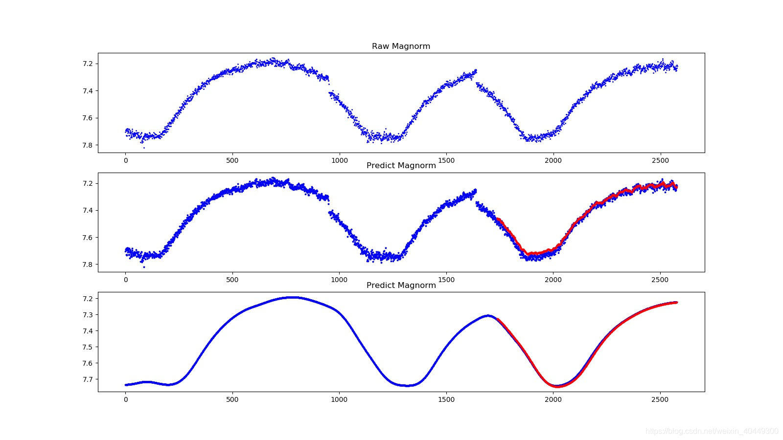
         说明：图1是原始曲线；图2蓝线是原始曲线，红点是在原始值上用LSTM预测值；图3是平滑以后的曲线，用LSTM预测的结果。

六、拓展材料

      1、时间序列平滑处理：https://blog.csdn.net/kylin_learn/article/details/85225761