毕设进度分享(二)
一、 图像融合网络Densefuse
基本原理
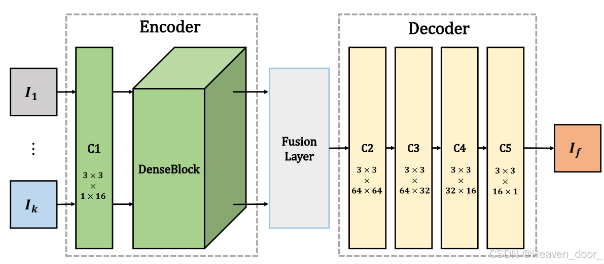
Densefuse是由编码网络和解码网络构建的新型深度学习架构,使用编码网络提取图像特征,通过解码网络得到融合后的图像。编码网络由卷积层和密集块构建,其中每一层的输出用作下一层的输入。因此编码网络中每一层的结果都被用来构建特征图。最后,通过融合策略和解码网络对融合后的图像进行重建,该网络包括 4 个 CNN 层。
如下图所示,输入图像统一记为I1I_1I1…IkI_kIk,原论文中假设输入图片都是预注册过的图片,因此不区分红外和可见光图片。编码器包含两部分( C1和Dense Block),用于提取深度特征。第一层( C1 )包含3 × 3滤波器提取粗略特征,密集块包含3个卷积层(每一层的输出级联作为下一层的输入),同样包含3 × 3滤波器。并且网络中,使用反射模式对输入图像进行pad。对于编码网络中的每个卷积层,特征图的输入通道数为16。
编码器的结构有两个优点。卷积操作的滤波器大小和步长分别为3 × 3和1。通过这种策略,输入图像可以是任意大小。其次,密集块结构可以在编码网络中尽可能多地保留深层特征,这种操作可以确保所有的显著特征都被用于融合策略。

下图是训练阶段网络结构,作者舍弃了融合层,先训练一个可以将输入图像复现的编码解码网络,此处训练使用的数据集理论上可能不受限制,只需要达到训练编码解码网络的效果即可。原文作者使用了coco2014数据集。
“这种训练策略的明显优势在于可以针对具体的融合任务设计合适的融合层。此外,为融合层的进一步发展留下了更大的空间。”个人理解为编码解码网络在这种训练策略下属于一种通用网络,最终融合效果取决于融合层策略的选择。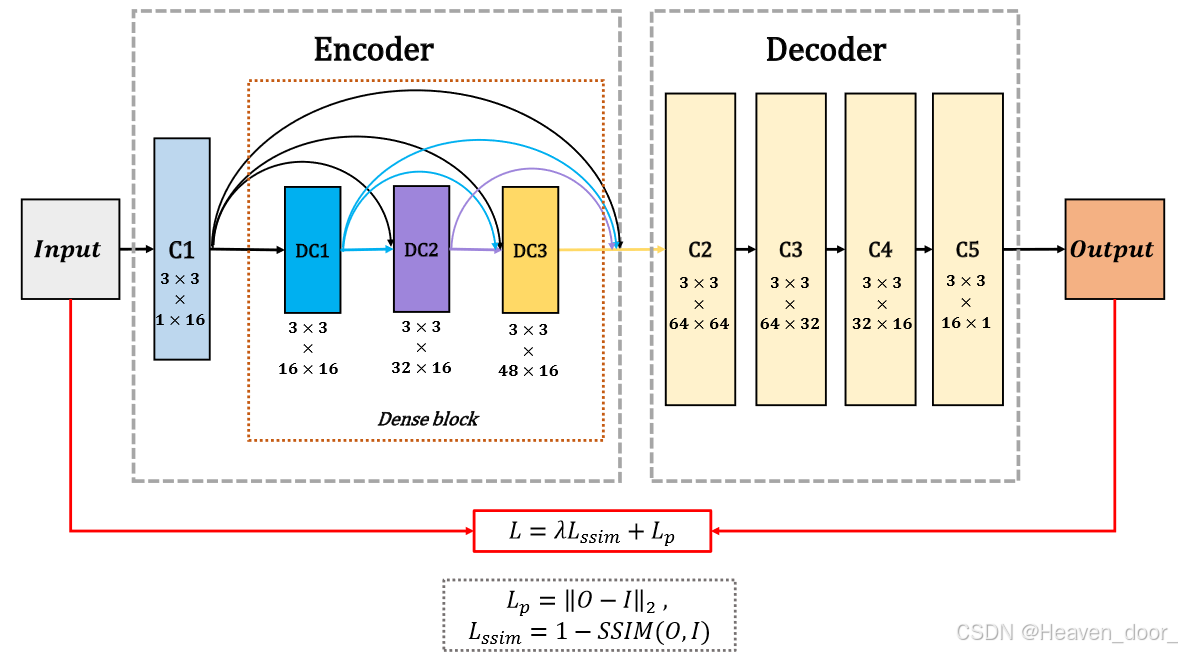
损失函数为LLL, 其中LpL_pLp为像素级损失,LssimL_{ssim}Lssim为结构相似性损失。像素损失和SSIM损失之间存在三个数量级的差异,因此在训练阶段,λ分别设置为1、10、100和1000。
如下为加性策略,ϕkm\phi_k^mϕkm为编码网络提取出的特征图,k为特征图索引,m代表特征图的数量。具体计算公式为
fm(x,y)=∑i=1kφim(x,y)f^m(x, y) = \sum_{i=1}^{k}φ^m_i (x, y)fm(x,y)=i=1∑kφim(x,y)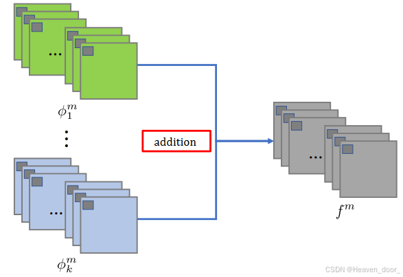
第二种融合策略基于l1范数和soft - max操作。该策略示意图如下图所示。其中C^i\hat C_iC^i是通过l1范数和基于块的平均算子算出来的。初始的CiC_iCi计算如下
Ci(x,y)=∣∣ϕi1:M(x,y)∣∣1C_i(x, y) = ||\phi^{1:M}_i (x, y)||_1Ci(x,y)=∣∣ϕi1:M(x,y)∣∣1
基于块平均的活动水平图C^\hat CC^
C^i(x,y)=∑a=−rr∑b=−rrCi(x+a,y+b)(2r+1)2\hat C_i(x, y)=\frac{\sum^{r}_{a=-r}\sum^{r}_{b=-r}C_i(x + a, y + b)}{(2r + 1)^2}C^i(x,y)=(2r+1)2∑a=−rr∑b=−rrCi(x+a,y+b)
其中r是块大小,作者设r=1
最终融合图
fm(x,y)=∑i=1kwi(x,y)×φim(x,y)f^m(x, y) = \sum^k_{i=1} w_i(x, y) × φ^m_i (x, y)fm(x,y)=i=1∑kwi(x,y)×φim(x,y)
wi(x,y)=C^i(x,y)∑n=1kC^n(x,y)w_i(x, y) =\frac{\hat C_i (x,y)}{\sum^k_{n=1}\hat C_n(x,y)}wi(x,y)=∑n=1kC^n(x,y)C^i(x,y)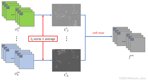
二、 代码分析
主要模块分6个
- args_fusion —— 存储超参数、路径和训练相关的设置
- fusion_strategy —— 定义融合策略函数
- net —— 定义卷积、密集卷积操作,定义密集块和整个网络
- utils —— 定义一系列操作,包括读取图片路径,图片读取、存储、数据集选择等
- train_densefuse —— 实现训练模型操作
- test_image —— 使用训练的模型进行图像融合
2.1 args_fusion
存储超参数及路径,主要包括
- 训练批数epochs
- 批量大小batch_size
- 读取数据集路径
- 图片指定大小
- 存储模型及损失值的路径
- ssim的权值
- 学习率
- 日志刷新间隔
- 恢复训练的路径,默认设置是None,每次从头训练
- 测试时使用的模型路径
    epochs = 4 #"number of training epochs, default is 2"
	batch_size = 4 #"batch size for training, default is 4"
	dataset = "F:\BaiduNetdiskDownload\coco2014\\train2014\\train2014"
	HEIGHT = 256
	WIDTH = 256

	save_model_dir = "models" #"path to folder where trained model will be saved."
	save_loss_dir = "models/loss"  # "path to folder where trained model will be saved."

	image_size = 256 #"size of training images, default is 256 X 256"
	cuda = 1 #"set it to 1 for running on GPU, 0 for CPU"
	seed = 42 #"random seed for training"
	ssim_weight = [1,10,100,1000,10000]
	ssim_path = ['1e0', '1e1', '1e2', '1e3', '1e4']

	lr = 1e-4 #"learning rate, default is 0.001"
	lr_light = 1e-4  # "learning rate, default is 0.001"
	log_interval = 5 #"number of images after which the training loss is logged, default is 500"
	resume = None  # 设置恢复训练的检查点路径。如果为 None,表示从头训练。
	resume_auto_en = None
	resume_auto_de = None
	resume_auto_fn = None

	# for test Final_cat_epoch_9_Wed_Jan__9_04_16_28_2019_1.0_1.0.model
	model_path_gray = "./models/densefuse_gray.model"
	model_path_rgb = "./models/densefuse_rgb.model"
2.2 fusion_strategy
模块中定义了addition_fusion加法策略、attention_fusion_weight基于注意力权重的融合策略两个方法。
加法策略直接把两个特征图取平均
def addition_fusion(tensor1, tensor2):
    return (tensor1 + tensor2)/2
基于权重图均值的注意力融合策略
def attention_fusion_weight(tensor1, tensor2):
    # avg, max, nuclear
    f_spatial = spatial_fusion(tensor1, tensor2)
    tensor_f = f_spatial
    return tensor_f
简单封装,没有真正功能
# spatial attention
def spatial_attention(tensor, spatial_type='sum'):
    if spatial_type == 'mean':
        spatial = tensor.mean(dim=1, keepdim=True)
    elif spatial_type == 'sum':
        spatial = tensor.sum(dim=1, keepdim=True)
    return spatial
把编码器输出的特征图按照 通道维度 进行求和或者求均值
def spatial_fusion(tensor1, tensor2, spatial_type='sum'):
    shape = tensor1.size()
    # calculate spatial attention 空间注意力
    spatial1 = spatial_attention(tensor1, spatial_type)
    spatial2 = spatial_attention(tensor2, spatial_type)

    # get weight map, soft-max 使用 softmax 类似的方法计算注意力权重,将两个张量对应位置的权重归一化。
    spatial_w1 = torch.exp(spatial1) / (torch.exp(spatial1) + torch.exp(spatial2) + EPSILON)
    spatial_w2 = torch.exp(spatial2) / (torch.exp(spatial1) + torch.exp(spatial2) + EPSILON)

    spatial_w1 = spatial_w1.repeat(1, shape[1], 1, 1)
    spatial_w2 = spatial_w2.repeat(1, shape[1], 1, 1)  # 保证权重图和输入图像维度一样才能逐元素相乘

    tensor_f = spatial_w1 * tensor1 + spatial_w2 * tensor2

    return tensor_f
把空间注意力处理过的特征图,用softmax类似方法求出权重,然后融合特征图由原图×权重得到。
2.3 net
共定义4个模块,ConvLayer定义卷积操作,DenseConv2d定义密集块卷积操作,DenseBlock定义密集块,DenseFuse_net汇总形成Densefuse网络。
class ConvLayer(torch.nn.Module):
    def __init__(self, in_channels, out_channels, kernel_size, stride, is_last=False):
        super(ConvLayer, self).__init__()
        reflection_padding = int(np.floor(kernel_size / 2))  # reflection_padding(反射填充)是根据卷积核的大小计算的填充量。卷积核大小的半径
        self.reflection_pad = nn.ReflectionPad2d(reflection_padding)  # 在输入的四周加上反射填充。
        self.conv2d = nn.Conv2d(in_channels, out_channels, kernel_size, stride)
        self.dropout = nn.Dropout2d(p=0.5)
        # 这个层会对输入特征图中的某些通道进行随机“丢弃”,丢弃概率为 p=0.5,即每个通道有 50% 的概率被丢弃。Dropout 是一种常用的正则化方法,能有效防止过拟合。
        self.is_last = is_last

    def forward(self, x):
        out = self.reflection_pad(x)
        out = self.conv2d(out)
        if self.is_last is False:
            # out = F.normalize(out)
            out = F.relu(out, inplace=True)  # inplace=True 表示在原地进行操作,节省内存。
            # out = self.dropout(out)
        return out
定义反射填充,卷积,dropout。前向操作使用反射填充,对于尺寸为3的卷积核,填充大小为1。对于非最后一层的网络,卷积后使用ReLu激活函数。
class DenseConv2d(torch.nn.Module):
    def __init__(self, in_channels, out_channels, kernel_size, stride):
        super(DenseConv2d, self).__init__()
        self.dense_conv = ConvLayer(in_channels, out_channels, kernel_size, stride)

    def forward(self, x):
        out = self.dense_conv(x)  # 传入x被ConvLayer中的forward使用
        out = torch.cat([x, out], 1)
        # 密集连接的核心操作。它将输入 x 和卷积操作得到的输出 out 沿着通道维度(维度 1)拼接。
        return out
将上述卷积操作实例化,密集块核心操作为将输入和输出拼接,作为下一个卷积层的输入。此处将卷积前后的特征图按通道拼接。
class DenseBlock(torch.nn.Module):
    def __init__(self, in_channels, kernel_size, stride):
        super(DenseBlock, self).__init__()
        out_channels_def = 16
        denseblock = []
        denseblock += [DenseConv2d(in_channels, out_channels_def, kernel_size, stride),
                       DenseConv2d(in_channels+out_channels_def, out_channels_def, kernel_size, stride),
                       DenseConv2d(in_channels+out_channels_def*2, out_channels_def, kernel_size, stride)]
        self.denseblock = nn.Sequential(*denseblock)
        # nn.Sequential 是一个容器模块,按顺序执行一系列操作。在这里,它将这三个卷积层按顺序组织起来,形成一个连续的模块。

    def forward(self, x):
        out = self.denseblock(x)
        return out
形成完整的密集块,因为有密集连接操作,所以后两层的输入通道分别叠加增加了前面层的输出通道。
nn.Sequential()可以将层集合,并形成顺序执行
class DenseFuse_net(nn.Module):
    def __init__(self, input_nc=1, output_nc=1):  # nc通道数
        super(DenseFuse_net, self).__init__()
        denseblock = DenseBlock
        nb_filter = [16, 64, 32, 16]  # 对应的通道数,用来调用
        kernel_size = 3
        stride = 1

        # encoder
        self.conv1 = ConvLayer(input_nc, nb_filter[0], kernel_size, stride)
        self.DB1 = denseblock(nb_filter[0], kernel_size, stride)

        # decoder
        self.conv2 = ConvLayer(nb_filter[1], nb_filter[1], kernel_size, stride)
        self.conv3 = ConvLayer(nb_filter[1], nb_filter[2], kernel_size, stride)
        self.conv4 = ConvLayer(nb_filter[2], nb_filter[3], kernel_size, stride)
        self.conv5 = ConvLayer(nb_filter[3], output_nc, kernel_size, stride)

    def encoder(self, input):
        x1 = self.conv1(input)
        x_DB = self.DB1(x1)
        return [x_DB]

    def fusion(self, en1, en2, strategy_type='addition'):
        f_0 = (en1[0] + en2[0])/2
        return [f_0]

    def decoder(self, f_en):
        x2 = self.conv2(f_en[0])
        x3 = self.conv3(x2)
        x4 = self.conv4(x3)
        output = self.conv5(x4)

        return [output]
网络结构如下图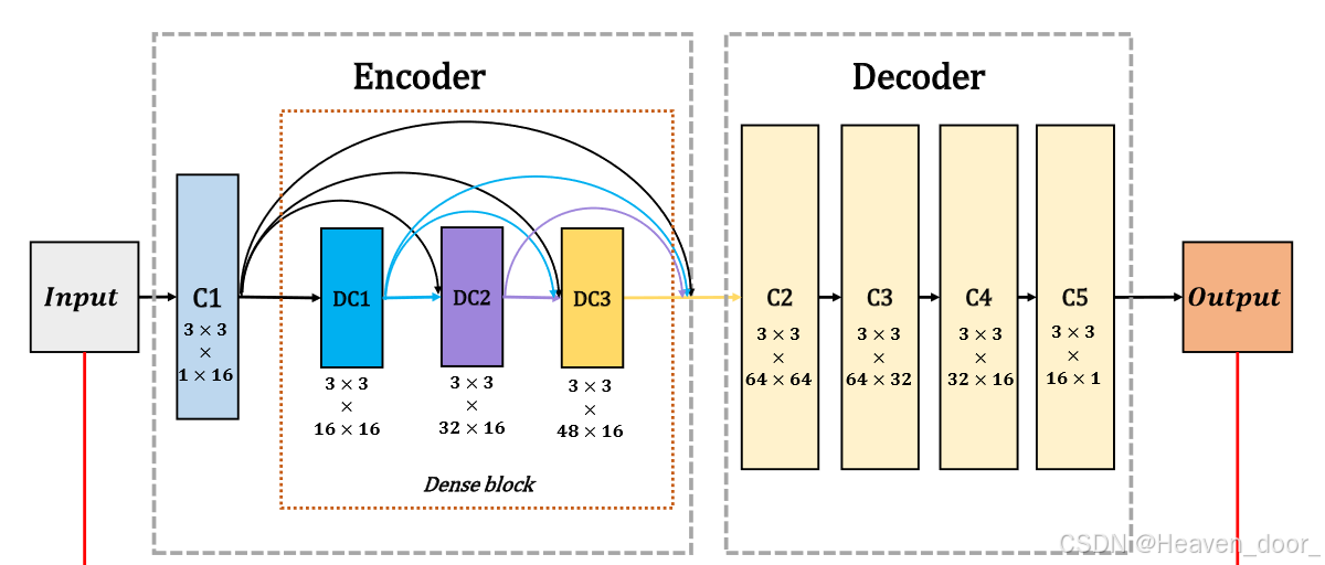
网络中不同层的细节如下图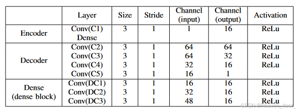
2.4 utils
包含定义函数12个
-
list_images(directory):
列出指定目录下的所有图像文件(.png, .jpg, .jpeg 格式),并返回它们的路径和去掉扩展名的文件名列表。 -
tensor_load_rgbimage(filename, size=None, scale=None, keep_asp=False):
加载图像并转换为RGB格式,支持根据指定的大小(size)或缩放比例(scale)调整图像大小,可以选择是否保持宽高比(keep_asp)。
返回:转换为PyTorch Tensor的图像。 -
get_image(path, height=256, width=256, mode=‘L’):
加载图像文件,根据需要进行大小调整,支持灰度图(‘L’)和RGB图像(‘RGB’)。
返回:加载后的图像,大小为height x width。 -
get_train_images_auto(paths, height=256, width=256, mode=‘RGB’):
批量加载训练图像,并转换为PyTorch Tensor。
参数:支持输入多个路径或单一路径,返回的图像会调整为指定的高度和宽度。 -
get_test_images(paths, height=None, width=None, mode=‘RGB’):
加载并转换测试图像,返回Tensor格式的图像。 -
tensor_save_rgbimage(tensor, filename, cuda=True):
将RGB图像从Tensor格式转换回图像文件并保存,支持CUDA设备和CPU。 -
tensor_save_bgrimage(tensor, filename, cuda=False):
将BGR格式的Tensor图像保存为文件,OpenCV使用的是BGR格式,函数通过将BGR顺序转换为RGB顺序后调用tensor_save_rgbimage来保存图像。 -
save_images(path, data):
保存图像数据为文件。使用OpenCV的imwrite函数将图像保存为指定路径。 -
gram_matrix(y):
计算Gram矩阵,表示不同通道之间的相关性。 -
matSqrt(x):
计算矩阵的平方根,利用奇异值分解(SVD)来实现。 -
load_dataset(image_path, BATCH_SIZE, num_imgs=None):
加载数据集,将图像路径按批次划分,并进行随机打乱,返回图像路径列表和批次数量。 -
colormap():
创建一个自定义的颜色映射。
2.5 test_densefuse
模型训练
main()中,读图像路径,选取训练图片数量,打乱图片路径,选取结构性损失权重,训练。
train()使用Adam优化器,用MSE损失函数衡量像素级差异,ssim为结构性相似指数。最终损失由MSE和SSIM损失加权表示。
2.6 test_image
使用的融合策略在此main中修改
从灰度图修改成RGB图,需要注意改
- 模型加载路径
- 测试图像路径
- 输入通道数
- 读图的后缀名(.jpg , .png)
三、 融合效果
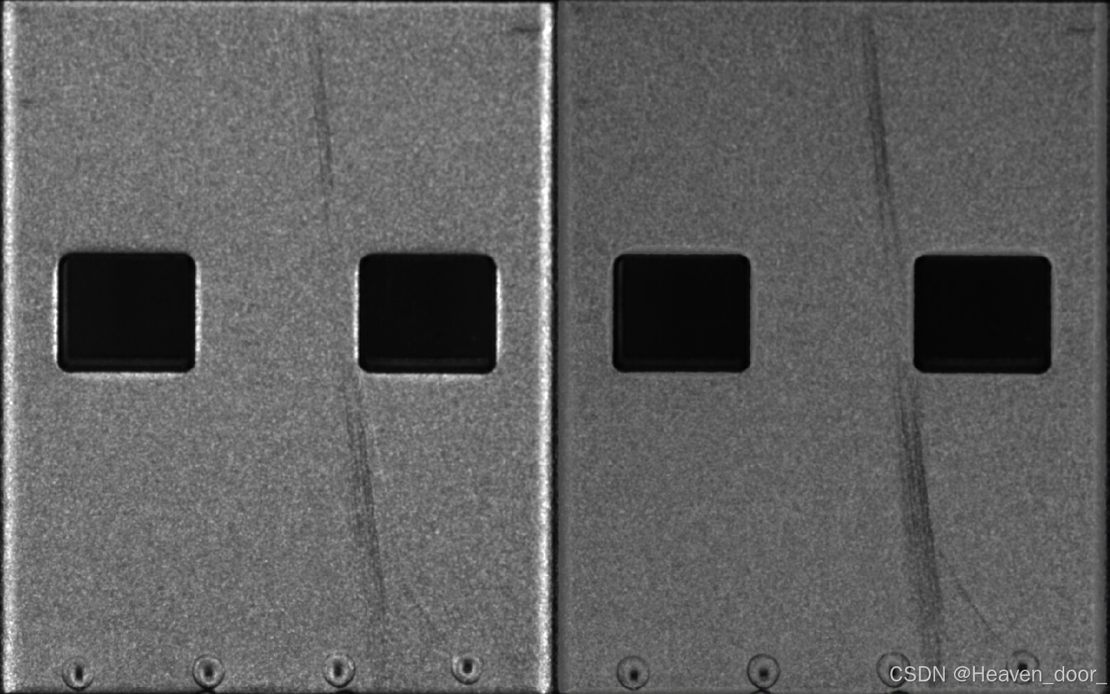
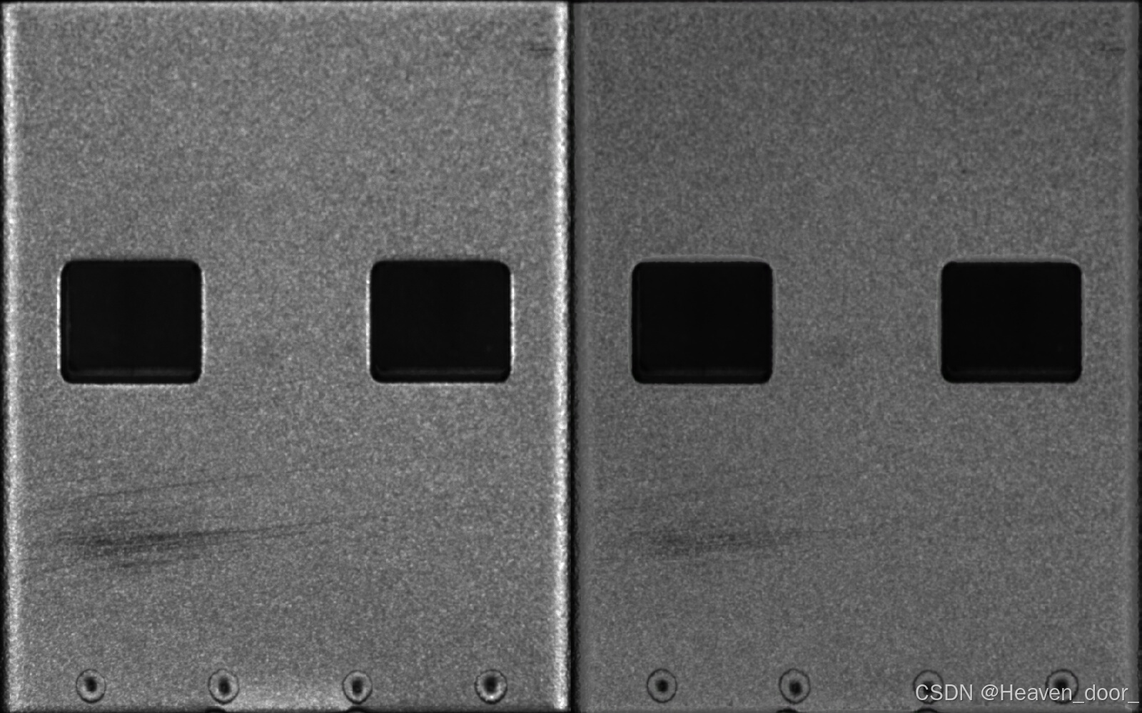
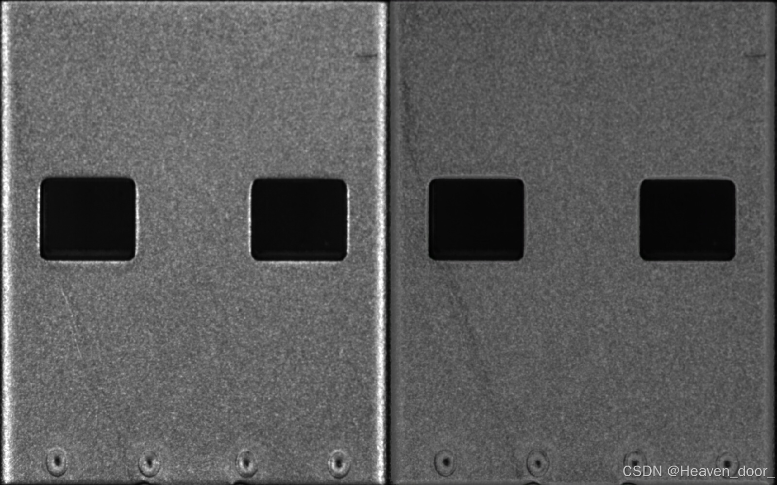
使用了多光源usb图像数据集,使用加性策略和空间注意力策略未展现过多差别。

有“AI”的1024 = 2048,欢迎大家加入2048 AI社区
更多推荐


 22
22 0
0- 0


 已为社区贡献1条内容

所有评论(0)