Matlab/Python各种概率分布函数，概率密度分布函数，概率分布函数拟合，绘图。伽马分布，威尔分布，正态分布，柯西分布，均匀分布。

Matlab/Python概率密度函数（pdf）和累计概率密度函数拟合（cdf）支持定制，包括不限于如下：（重现期极值计算）

1. Beta Distribution (Beta 分布)
2. Binomial Distribution (二项分布)
3. Birnbaum-Saunders Distribution (伯恩鲍姆-桑德斯分布)
4. Burr Distribution (伯尔分布)
5. Exponential Distribution (指数分布)
6. Extreme Value Distribution (极值分布)
7. Gamma Distribution (gamma 分布)
8. Generalized Extreme Value Distribution (广义极值分布)
9. Generalized Pareto Distribution (广义帕累托分布)
10. Half Normal Distribution (半正态分布)
11. Inverse Gaussian Distribution (逆高斯分布)
12. Kernel Distribution (核分布)
13. Logistic Distribution (逻辑分布)
14. Loglogistic Distribution (对数逻辑分布)
15. Lognormal Distribution (对数正态分布)
16. Nakagami Distribution (Nakagami 分布)
17. Negative Binomial Distribution (负二项分布)
18. Normal Distribution (正态分布)
19. Poisson Distribution (泊松分布)
20. Rayleigh Distribution (瑞利分布)
21. Rician Distribution (莱斯分布)等
22. Stable Distribution (稳定分布)
23. t Location-Scale Distribution (t 位置尺度分布)
24. Weibull Distribution (威布尔分布)
    等约100种，详情查列表

在Matlab和Python中，处理各种概率分布函数（PDF）和累积分布函数（CDF），以及进行分布拟合和绘图是非常常见的任务。以下是针对您提到的几种分布（伽马分布、威尔分布、正态分布等）的基本操作方法示例。

在Matlab中

对于大多数分布，Matlab提供了fitdist函数用于数据拟合，pdf和cdf函数来计算特定点的概率密度和累积概率值，以及plot或histogram结合pdf绘制图形。

% 示例：伽马分布拟合并绘图
data = gamrnd(1,1,100,1); % 生成随机数作为样本数据
pd = fitdist(data,'Gamma'); % 拟合伽马分布
x = linspace(min(data),max(data));
y_pdf = pdf(pd,x); % 计算概率密度
y_cdf = cdf(pd,x); % 计算累积概率

figure;
subplot(2,1,1); plot(x,y_pdf); title('Gamma PDF');
subplot(2,1,2); plot(x,y_cdf); title('Gamma CDF');

在Python中

使用SciPy库可以方便地进行类似的操作。下面以伽马分布为例：

import numpy as np
import matplotlib.pyplot as plt
from scipy.stats import gamma
from scipy.optimize import curve_fit

# 生成随机样本
data = gamma.rvs(a=1, size=100)

# 定义拟合函数
def gamma_pdf(x, a, loc, scale):
    return gamma.pdf(x, a, loc, scale)

params, _ = curve_fit(gamma_pdf, np.arange(len(data)), data)
a, loc, scale = params

x = np.linspace(min(data), max(data), 100)
pdf_fitted = gamma.pdf(x, a=a, loc=loc, scale=scale)
cdf_fitted = gamma.cdf(x, a=a, loc=loc, scale=scale)

plt.figure(figsize=(12, 6))
plt.subplot(1, 2, 1)
plt.plot(x, pdf_fitted, label='Fitted Gamma PDF')
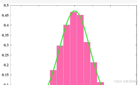
plt.hist(data, density=True, alpha=0.5, label='Data Histogram')
plt.legend()

plt.subplot(1, 2, 2)
plt.plot(x, cdf_fitted, label='Fitted Gamma CDF')
plt.legend()
plt.show()

以上代码分别展示了如何在Matlab和Python中对数据进行伽马分布拟合，并绘制其概率密度函数（PDF）和累积分布函数（CDF）。其他分布的操作方式类似，只需更改相应的分布名称及其参数即可。对于更多类型的分布，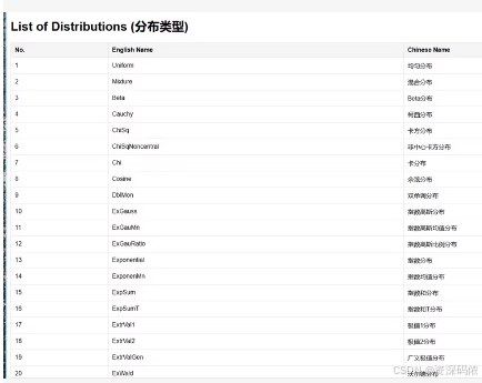

这里展示的是一个包含多种概率分布的列表。为了帮助您更好地理解和使用这些分布，我将提供一些基本示例代码，分别在Matlab和Python中实现对几种常见分布的概率密度函数（PDF）和累积分布函数（CDF）的计算与绘图。

在Matlab中

首先，我们选择几个常见的分布进行示例：

% 示例：正态分布、伽马分布和威布尔分布的PDF和CDF绘制

% 正态分布
mu = 0; % 均值
sigma = 1; % 标准差
x_normal = linspace(mu - 3*sigma, mu + 3*sigma, 100);
pdf_normal = normpdf(x_normal, mu, sigma);
cdf_normal = normcdf(x_normal, mu, sigma);

% 伽马分布
a = 2; % 形状参数
b = 1; % 尺度参数
x_gamma = linspace(0, 10, 100);
pdf_gamma = gampdf(x_gamma, a, b);
cdf_gamma = gamcdf(x_gamma, a, b);

% 威布尔分布
k = 1.5; % 形状参数
lambda = 1; % 尺度参数
x_weibull = linspace(0, 10, 100);
pdf_weibull = wblpdf(x_weibull, k, lambda);
cdf_weibull = wbllike(x_weibull, k, lambda);

% 绘制图形
figure;
subplot(3, 2, 1); plot(x_normal, pdf_normal); title('Normal PDF');
subplot(3, 2, 2); plot(x_normal, cdf_normal); title('Normal CDF');
subplot(3, 2, 3); plot(x_gamma, pdf_gamma); title('Gamma PDF');
subplot(3, 2, 4); plot(x_gamma, cdf_gamma); title('Gamma CDF');
subplot(3, 2, 5); plot(x_weibull, pdf_weibull); title('Weibull PDF');
subplot(3, 2, 6); plot(x_weibull, cdf_weibull); title('Weibull CDF');

在Python中

接下来，我们使用Python中的SciPy库来实现同样的功能：

import numpy as np
import matplotlib.pyplot as plt
from scipy.stats import norm, gamma, weibull_min

# 正态分布
mu = 0
sigma = 1
x_normal = np.linspace(mu - 3*sigma, mu + 3*sigma, 100)
pdf_normal = norm.pdf(x_normal, mu, sigma)
cdf_normal = norm.cdf(x_normal, mu, sigma)

# 伽马分布
a = 2
b = 1
x_gamma = np.linspace(0, 10, 100)
pdf_gamma = gamma.pdf(x_gamma, a, scale=b)
cdf_gamma = gamma.cdf(x_gamma, a, scale=b)

# 威布尔分布
k = 1.5
lambda_ = 1
x_weibull = np.linspace(0, 10, 100)
pdf_weibull = weibull_min.pdf(x_weibull, k, scale=lambda_)
cdf_weibull = weibull_min.cdf(x_weibull, k, scale=lambda_)

# 绘制图形
plt.figure(figsize=(12, 8))
plt.subplot(3, 2, 1)
plt.plot(x_normal, pdf_normal)
plt.title('Normal PDF')

plt.subplot(3, 2, 2)
plt.plot(x_normal, cdf_normal)
plt.title('Normal CDF')

plt.subplot(3, 2, 3)
plt.plot(x_gamma, pdf_gamma)
plt.title('Gamma PDF')

plt.subplot(3, 2, 4)
plt.plot(x_gamma, cdf_gamma)
plt.title('Gamma CDF')

plt.subplot(3, 2, 5)
plt.plot(x_weibull, pdf_weibull)
plt.title('Weibull PDF')

plt.subplot(3, 2, 6)
plt.plot(x_weibull, cdf_weibull)
plt.title('Weibull CDF')

plt.tight_layout()
plt.show()

以上代码展示了如何在Matlab和Python中计算并绘制正态分布、伽马分布和威布尔分布的概率密度函数（PDF）和累积分布函数（CDF）。您可以根据需要调整参数或选择其他分布类型进行类似的处理。
Matlab/Python各种概率分布函数，概率密度分布函数，概率分布函数拟合，绘图。伽马分布，威尔分布，正态分布，柯西分布，均匀分布