opencv图像直方图
所以在每⼀个的区域中, 直⽅图会集中在某⼀个小的区域中)。对于每个⼩块来说,如果直⽅图中的 bin 超过对⽐度的上限的话,就把其中的像素点均匀分散到其他 bins 中,然后在进⾏直⽅图均衡化。这种⽅法提⾼图像整体的对⽐度,特别是有⽤数据的像素值分布⽐较接近时,在曝光过度或不⾜的图像中可以更好的突出细节。掩膜是⽤选定的图像、图形或物体,对要处理的图像进⾏遮挡,来控制图像 处理的区域。掩膜是由0和1组
直方图
可以将直方图视为图形或绘图,从而可以总体了解图像的强度分布。它是在X轴上具有像素值,在Y轴上具有图像中相应像素数的图。可以直观地了解图像的对比度,亮度,强度分布等。直方图的左侧区域显示图像中较暗像素的数量,右侧区域则显示明亮像素的数量。
OpenCV中的直方图计算
cv.calcHist(images,channels,mask,histSize,ranges [,hist [,accumulate]])- images:它是uint8或float32类型的源图像。它应该放在方括号中,即“ [img]”。
- channels:以方括号给出,是计算直方图通道的索引。如果输入为灰度图像,则其值为[0]。对于彩色图像,可以传递[0],[1]或[2]分别计算蓝色,绿色或红色通道的直方图。
- mask:图像掩码。完整图像的直方图,将其指定为“无”。如果要查找图像特定区域的直方图,需要创建一个掩码图像并将其作为掩码。
- histSize:表示BIN计数。需要放在方括号中。对于全尺寸,我们通过[256]。
- ranges:像素值范围,通常为[0,256]
def test():
    img = cv.imread('cat.jpg')
    color = ('b', 'g', 'r')
    for i, col in enumerate(color):
        histr = cv.calcHist([img], [i], None, [256], [0, 256])
        plt.plot(histr, color=col)
        plt.grid(True)
        plt.xlim([0, 256])
plt.show() 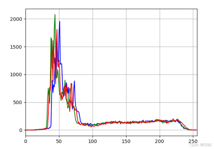
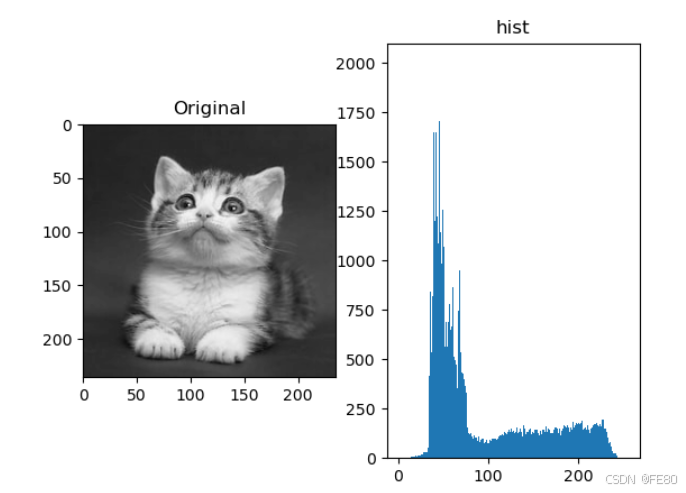
Matplotlib绘制直方图
def test():
    img = cv.imread('cat.jpg', 0)
    plt.subplot(121),plt.imshow(img,cmap="gray"),plt.title('Original')
    # ravel() 展成一维数组
    plt.subplot(122),plt.hist(img.ravel(), 256, [0, 256]),plt.title('hist')
    plt.show()
掩膜
掩膜是⽤选定的图像、图形或物体,对要处理的图像进⾏遮挡,来控制图像 处理的区域。在数字图像处理中,我们通常使⽤⼆维矩阵数组进⾏掩膜。掩膜是由0和1组成⼀个⼆进制图像,利⽤该掩膜图像要处理的图像进⾏掩膜,其中1值的区域被处理,0值区域被屏蔽,不会处理。
def test():
    # 1. 直接以灰度图的⽅式读⼊
    img = cv.imread('cat.jpg', 0)
    # 2. 创建蒙版
    mask = np.zeros(img.shape[:2], np.uint8)
    mask[25:140, 55:190] = 255
    # 3.掩模
    masked_img = cv.bitwise_and(img, img, mask=mask)
    # 4. 统计掩膜后图像的灰度图
    mask_histr = cv.calcHist([img], [0], mask, [256], [1, 256])
    # 5. 图像展示
    mpl.rcParams['font.family'] = 'SimHei'
    fig, axes = plt.subplots(nrows=2, ncols=2, figsize=(10, 8))
    axes[0, 0].imshow(img, cmap="gray"),axes[0, 0].set_title("Original")
    axes[0, 1].imshow(mask, cmap="gray"),axes[0, 1].set_title("mask")
    axes[1, 0].imshow(masked_img, cmap="gray"),axes[1, 0].set_title("masked_img")
    axes[1, 1].plot(mask_histr),axes[1, 1].grid(),axes[1, 1].set_title("mask_histr")
    plt.show()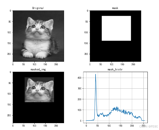
直方图均衡化
“直⽅图均衡化”是把原始图像的灰度直⽅图从⽐较集中的某个灰度区间变成在更⼴泛灰度范围内的分布。直⽅图均衡化就是对图像进⾏⾮线性拉伸,重新分配图像像素值,使⼀定灰度范围内的像素数量⼤致相同。这种⽅法提⾼图像整体的对⽐度,特别是有⽤数据的像素值分布⽐较接近时,在曝光过度或不⾜的图像中可以更好的突出细节。
# img 灰度图像
dst = cv.equalizeHist(img)
自适应的直方图均衡化
此时, 整幅图像会被分成很多⼩块,这些⼩块被称为“tiles”(在 OpenCV 中 tiles 的 ⼤⼩默认是 8x8),然后再对每⼀个⼩块分别进⾏直⽅图均衡化。 所以在每⼀个的区域中, 直⽅图会集中在某⼀个小的区域中)。如果有噪声的话,噪声会被放⼤。为了避免这种情况的出现要使⽤对⽐度限制。对于每个⼩块来说,如果直⽅图中的 bin 超过对⽐度的上限的话,就把其中的像素点均匀分散到其他 bins 中,然后在进⾏直⽅图均衡化。最后为了去除每⼀个⼩块之间的边界,再使⽤双线性差值,对每⼀⼩块进⾏拼接。
cv.createCLAHE(clipLimit, tileGridSize)参数:clipLimit: 对比度限制,默认是40 tileGridSize: 分块的大小,默认为8 ∗ 8
def test():
    img = cv.imread('cat.jpg',0)
    # 直方图均衡化
    dst = cv.equalizeHist(img)
    # 自适应均衡化
    clahe = cv.createCLAHE(clipLimit=2.0, tileGridSize=(8,8))
    clahe_img = clahe.apply(img)
    plt.figure(figsize=(10,5))
    plt.subplot(131),plt.imshow(img, cmap="gray"),plt.title('Original')
    plt.subplot(132),plt.imshow(dst, cmap="gray"),plt.title('dst')
    plt.subplot(133),plt.imshow(clahe_img, cmap="gray"),plt.title('clahe_img')
    plt.show()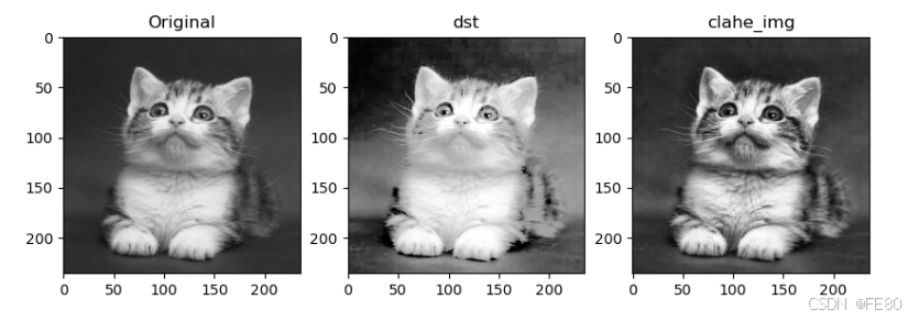

有“AI”的1024 = 2048,欢迎大家加入2048 AI社区
更多推荐

 25
25 0
0- 0


 已为社区贡献3条内容

所有评论(0)