评价指标

准确率/精确率/召回率

	Positive (预测到的正例)	Negative (预测到的反例)
True (预测结果为真)	TP	TN
False (预测结果为假)	FP	FN

争对正案例的计算：

1、准确率计算方式（ACC）：$Acc=\frac{TP+TN}{TP+TN+FP+FN}$
2、精确率计算方式（Precision）：$\frac{TP}{TP+FP}$
3、召回率计算方式（Recall）：$\frac{TP}{TP+FN}$
4、F1计算方式：$\frac{2\times Precision\times Recall}{Precision+Recall}$

指标	优点	缺点
准确率	- 直观且易理解	- 在类别不平衡的情况下可能误导模型评估
精确率	- 衡量预测为正类的样本中，实际为正类的比例；适用于避免假阳性	- 可能忽视召回率，导致漏掉正类样本（假阴性）
召回率	- 衡量模型对正类样本的识别能力；适用于避免假阴性	- 可能导致精确率较低，增加误报（假阳性）
F1 分数	- 平衡精确率和召回率，适用于不平衡的任务	- 不能单独反映精确率或召回率，可能不适用于需要单独关注某一项的场景

BLEU

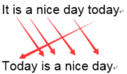
BLEU 采用一种N-gram的匹配规则，原理比较简单，就是比较译文和参考译文之间n组词的相似的一个占比
原文：今天天气不错
机器译文：It is a nice day today
人工译文：Today is a nice day
1-gram:

命中5个词，那么计算得到匹配度为：$5/6$
3-gram:

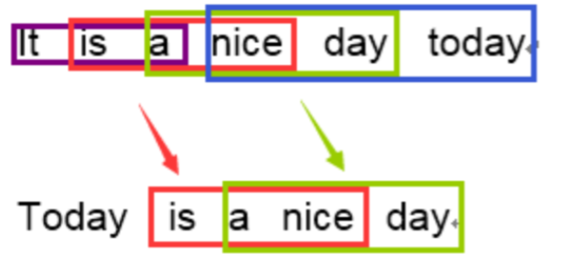
计算得到匹配度为：$2/4$

在通过结合召回率和惩罚因子之后得到BLEU计算公式为：

$$BLEU=BP\times exp(\sum _{n=1}^N{W}_{n}log{P}_n)$$

使用例子，直接使用第三方库sacrebleu

import sacrebleu
hyps = ['我有一个帽衫', '大大的帽子']
refs = ['你好，我有一个帽衫', '帽子大大的']
bleu = sacrebleu.corpus_bleu(hyps, [refs], tokenize='zh')
print(float(bleu.score))
# 59.809989126151606

Loss Function

Cross-Entropy Loss(交叉熵损失)

交叉熵损失用于分类任务，它度量的是预测概率分布与真实标签分布之间的差异。通常用于多分类问题。交叉熵损失公式（多分类）如下：

$$L=-\sum _{i=1}^N{y}_{i}log(p_i)$$

其中$N$为类别数量，$y_i$真实标签数据，$p_i$模型预测概率。二分类交叉熵损失为：$Loss=-[ylog(p)+(1-y)log(1-p)]$
在pytorch中对于交叉熵损失函数主要参数：

• 1、label_smoothing (float, optional)：通过平滑标签的方式来避免模型过度自信，提高模型的泛化能力并缓解类别不平衡问题的技术。假设模型有 C 个类别，标签为 y，真实标签的平滑值为 ε，则：对于真实类别 y = 1，标签值变为 1 - ε；对于其他类别 y ≠ 1，标签值变为 ε / (C - 1)
• 2、ignore_index (int, optional)：忽略某些特定的标签，通常用于标记某些数据的特殊情况，如填充（padding）区域、无效标签或其他不需要参与损失计算的标签
• 3、reduction (str, optional)：‘none’、‘mean’ 和 'sum’分别表示对最后 不汇总、平均值、求和

⭐值得注意的是，在pytorch的交叉熵损失里面已经计算了softmax/sigmoid，所以模型输出如果用交叉熵损失函数就不需要用softmax/sigmoid处理

Mean Squared Error(均方误差)

均方误差损失用于回归任务，度量预测值与真实值之间的差异。MSE 计算的是预测值和实际值的平方误差的平均值。MSE 公式：

$$L=\frac{1}{N}\sum _{i=1}^N(y_i-p_i{)}^2$$

其中$N$为类别数量，$y_i$真实标签数据，$p_i$模型预测概率

例子：比如说预测类别（假设为3），模型输出之后通过sigmoid/softmax处理之后得到：

预测	真实
0.3 0.3 0.4	0 0 1 (A)
0.3 0.4 0.3	0 1 0 (B)
0.1 0.2 0.7	1 0 0 ©

均方误差计算：$\frac{(0.3-0{)}^2+(0.3-0{)}^2+(0.4-1{)}^2+...}{3}=0.81$
交叉熵计算：$\frac{-(0\times log0.3+0\times log0.3+1\times log0.4+...)}{3}=1.37$

Focal Loss

**Focal Loss**主要用于处理样本失衡问题（样本里面标签不平衡问题，比如说目标识别，可能会得到很多框，但是可能只要一个框是所需的），其原理也很简单可以直接在原交叉熵基础上补充一个 因子即可。

$$FL(p_t)=-{\alpha }_t(1-p_t{)}^{\gamma }log(p_t)$$

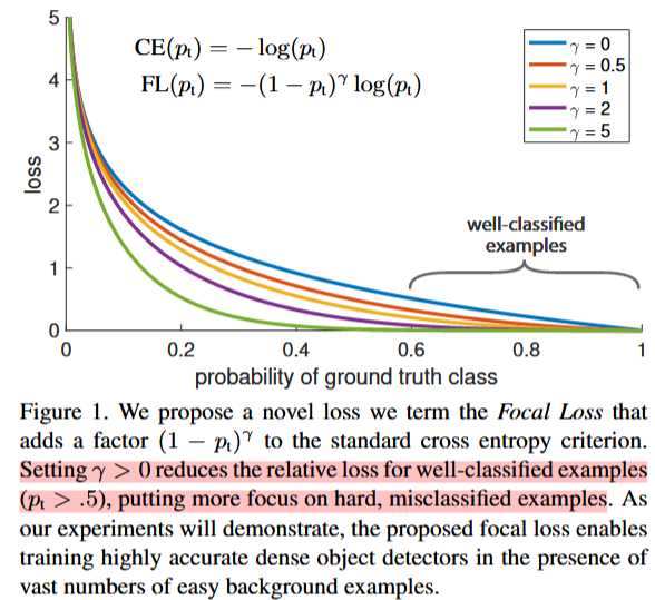
$\gamma$：调节因子，用于控制对易分类样本的惩罚程度。它是一个非负实数，通常设置为大于 0 的值。当$\gamma$>0 时，随着$p_t$的增加，$(1-p_t{)}^{\gamma }$的值会迅速减小，从而降低易分类样本的损失值。这样可以使得模型更加关注那些难以分类的样本。
$\alpha$: 平衡因子，用于调整正类和负类之间的权重。它是一个可调参数，通常设置为$\alpha$对于正类和 1−$\alpha$对于负类。当数据集中正负样本数量不均衡时，可以通过调整$\alpha$来平衡两类样本的贡献。例如，在一个正负样本比例为 1:9 的数据集中，可以将$\alpha$设置为 0.9，以增加正类样本的权重

import torch
import torch.nn as nn
import torch.nn.functional as F

class FocalLoss(nn.Module):
    """Focal Loss implementation."""
    
    def __init__(self, gamma=1.5, alpha=0.25):
        super().__init__()
        self.gamma = gamma
        self.alpha = alpha

    def forward(self, pred, label, mask_labels=None):
        """Calculates focal loss with optional mask_labels."""
        loss = F.binary_cross_entropy_with_logits(pred, label, reduction='none')
        pred_prob = pred.sigmoid()
        p_t = label * pred_prob + (1 - label) * (1 - pred_prob)
        loss *= (1.0 - p_t) ** self.gamma
        
        if self.alpha > 0:
            loss *= label * self.alpha + (1 - label) * (1 - self.alpha)
        
        if mask_labels is not None:
            loss *= mask_labels.float()
            return loss.sum() / mask_labels.sum()
        
        return loss.mean()

if __name__ == '__main__':
    h, w = 500, 500
    labels_parent = torch.randint(0, 2, (h, w), dtype=torch.float32)
    tmp_labels = torch.zeros(1000, 1000)
    tmp_labels[:h, :w] = labels_parent
    tmp_labels_mask = torch.zeros(1000, 1000)
    tmp_labels_mask[:h, :w] = 1 
    pred = torch.randn(1, 1000, 1000)

    focal_loss = FocalLoss()
    loss = focal_loss(pred, tmp_labels.unsqueeze(0), tmp_labels_mask)
    print(loss)

L1 loss

L1 loss：算预测值与真实值之间的绝对差值来衡量模型的预测误差，公式为：$L=\frac{1}{N}{\sum }_{i=1}^N|y_i-{\hat{y}}_i|$

Huber Loss

Huber Loss用于回归任务的损失函数，它结合了均方误差（MSE）和绝对误差（MAE）的优点，可以减少对异常值（outliers）的敏感性，同时保持较好的梯度性质

$$\mathrm{Huber}\mathrm{Loss}=\{\begin{array}{llcc}\frac{1}{2}(y-\hat{y}{)}^2& \mathrm{if}|y-\hat{y}|\le \delta & & \\ \delta \ast (|y-\hat{y}|-\frac{1}{2}\ast \delta )& \mathrm{otherwise}& & \end{array}$$

参考

1、https://pytorch.org/docs/stable/generated/torch.nn.CrossEntropyLoss.html
2、https://pytorch.org/docs/stable/generated/torch.nn.L1Loss.html#torch.nn.L1Loss
3、Focal Loss for Dense Object Detection
4、https://blog.csdn.net/zhang2010hao/article/details/84559971
5、https://www.big-yellow-j.top/posts/2025/01/01/evaluation-lossfunction.html