废话一下

本来是想研究HWGAT模型的，之前也说要发yolo具体模型学习情况，结果就是一看模型就还是有点头疼，简单模型可能还可以看完，这些模型却实在看不动，意识到基础不是很牢固，很大知识点没那么清晰，所以又拿起了李沐的《动手学深度学校》。后面就先持续更新这部分的内容，解释可能不会太多，理解还不太深刻，主要是一种记录，代码也不会跟书完全一样。

环境安装

conda create -n d2l python=3.9 -y
conda activate d2l
pip install torch==1.12.0 -i  https://pypi.tuna.tsinghua.edu.cn/simple
pip install torchvision==0.13.0 -i  https://pypi.tuna.tsinghua.edu.cn/simple
pip install jupyter -i  https://pypi.tuna.tsinghua.edu.cn/simple
jupyter-notebook

预备知识

torch的一些基础预处理

import torch

生成0到n-1的数据

参数

start (Number) – the starting value for the set of points. Default: 0.

end (Number) – the ending value for the set of points

step (Number) – the gap between each pair of adjacent points. Default: 1.

起始数，默认为0

结尾数，不包括自己

步长，默认为1

x=torch.arange(12)
x

这个叫做张量，数学上叫向量

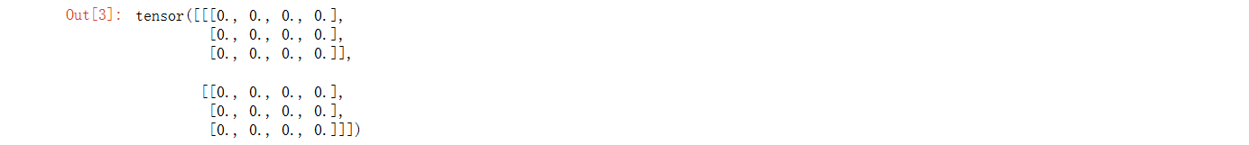
生成全0数据

参数

size (int…) – a sequence of integers defining the shape of the output tensor. Can be a variable number of arguments or a collection like a list or tuple.

长度

x1=torch.zeros((2,3,4))
x1

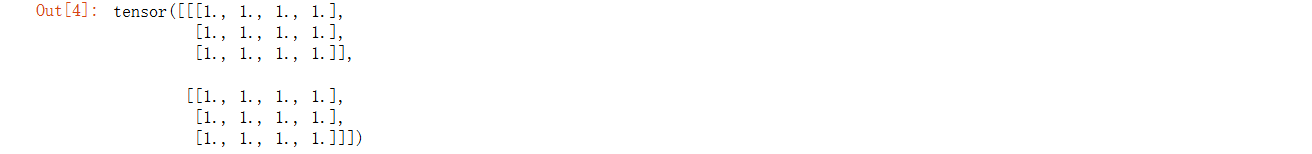
生成全是1的数据

参数

size (int…) – a sequence of integers defining the shape of the output tensor. Can be a variable number of arguments or a collection like a list or tuple.

长度

x2=torch.ones((2,3,4))
x2

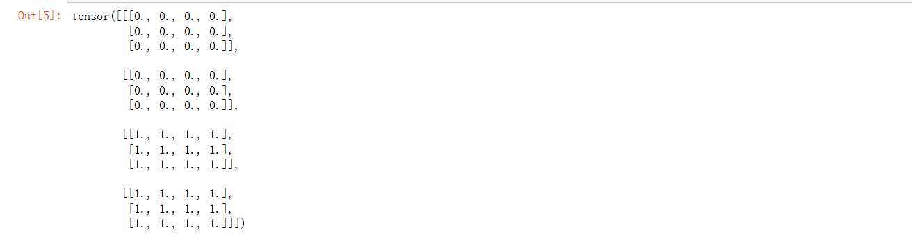
合并数据

参数

tensors (sequence of Tensors) – any python sequence of tensors of the same type. Non-empty tensors provided must have the same shape, except in the cat dimension.

dim (int, optional) – the dimension over which the tensors are concatenated

张量序列

合并维度

x=torch.cat((x1,x2),0)
x

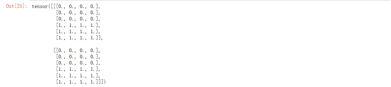
y=torch.cat((x1,x2),1)
y

生成随机数均值为0，方差为1

参数

size (int…) – a sequence of integers defining the shape of the output tensor. Can be a variable number of arguments or a collection like a list or tuple.

大小

y=torch.randn(2,3)
y

生成我想要的张量

a=torch.tensor([[2,2],[4,3]])
a

获取形状

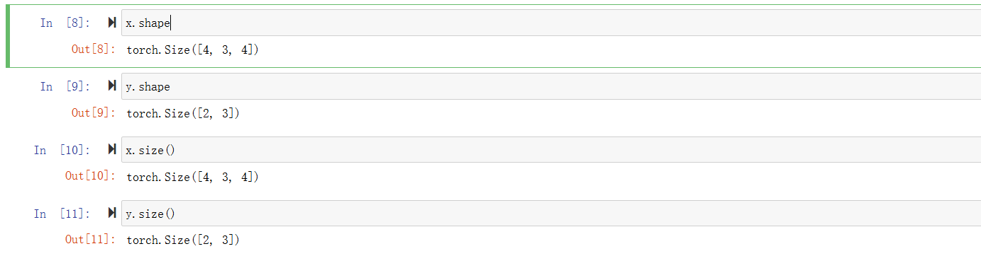
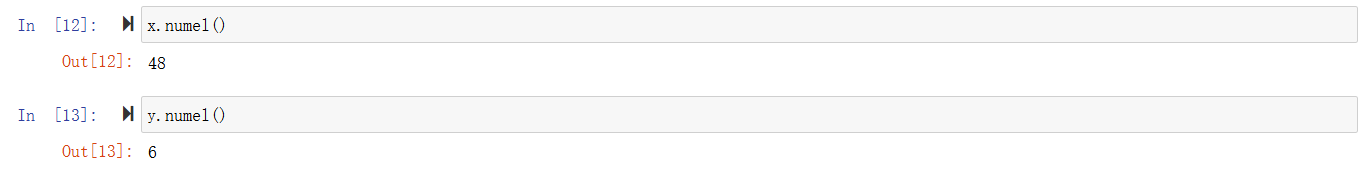
获取数量

改变形状

参数

input (Tensor) – the tensor to be reshaped

shape (tuple of int) – the new shape

数据

需要改变的形状

x.reshape(6,8)

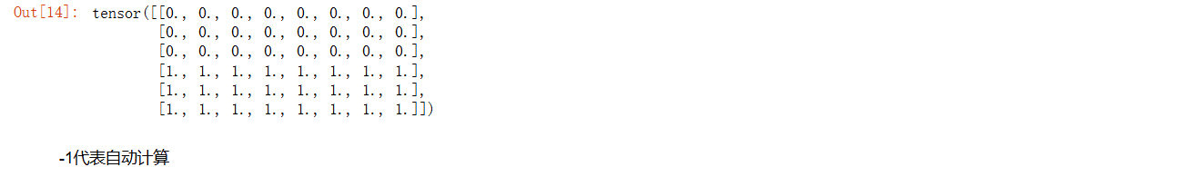
-1代表自动计算

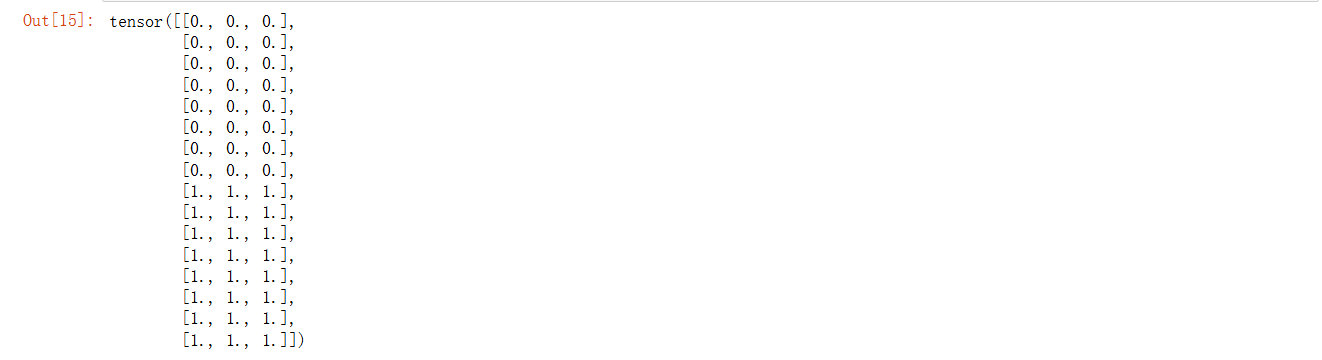
x.reshape(-1,3)

数字计算

在相同形状的张量上进行按位运算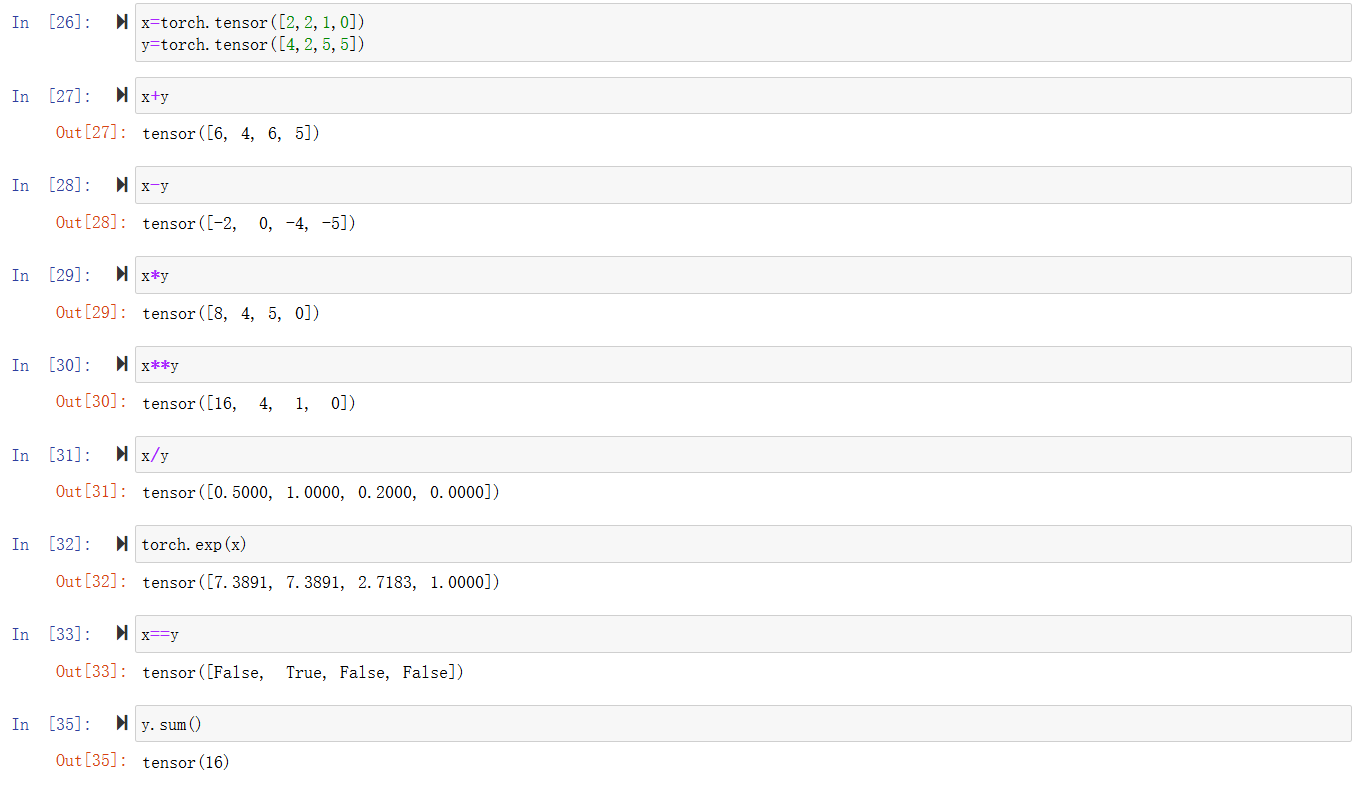

广播机制

当两个张量形状不同时，通过适当扩展使得两个张量形状相同

x=torch.tensor([1,2])
y=torch.arange(3).reshape((3,1))
x,y

x+y

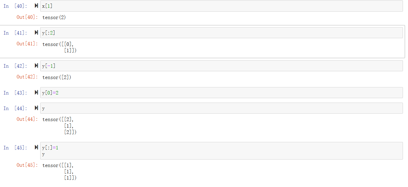
切片和索引

节省内存

id可以获取到内存的地址，用于验证y=y+x中y是否被分配了新的内存

before=id(y)
y=y+x
id(y)==before

我们可以通过y[:]实现原地更新或者使用y+=x

before=id(y)
y[:]=y+x
id(y)==before

before=id(y)
y+=x
id(y)==before

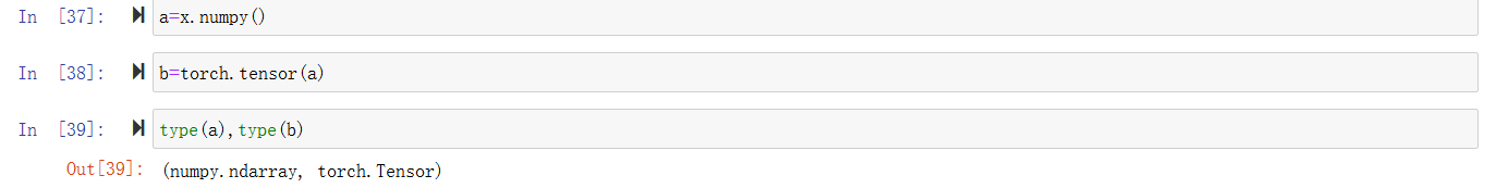
转换成numpy类型

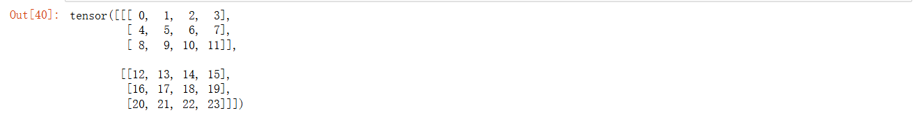
线性代数

A=torch.arange(24).reshape((2,3,4))
A

降维

通过sum降低到一维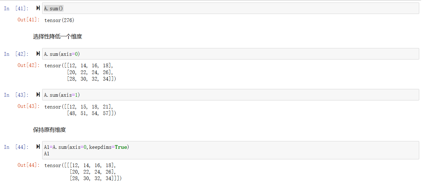

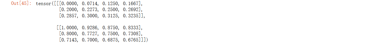
使得通过广播机制可以实现计算

A/A1

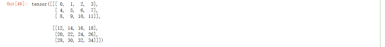
不降低维度计算总和

A.cumsum(axis=0)

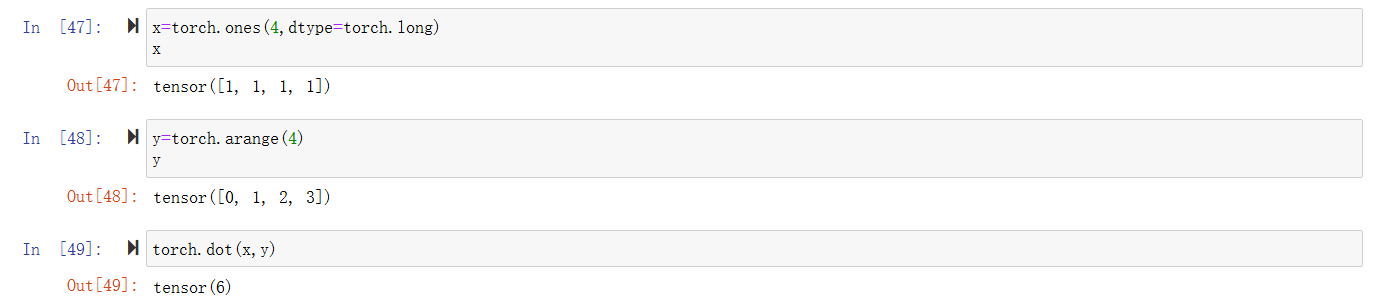
点积

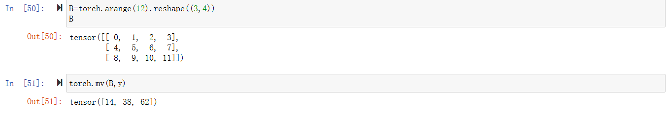
向量与矩阵乘

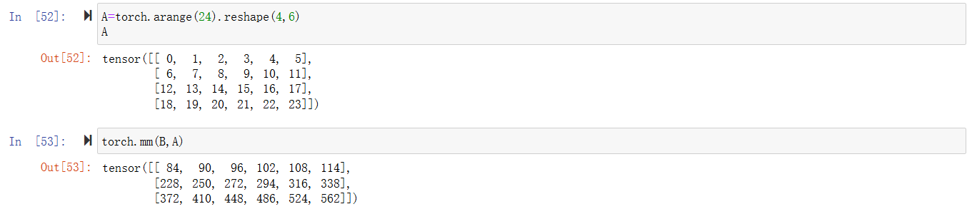
矩阵与矩阵乘

范数

L2范数特例欧几里得算法

u=torch.tensor([3.0,4.0])
torch.norm(u)

L1范数是绝对值相加

torch.abs(u).sum()

矩阵L2范数，将每一行的向量单独取L2范数合成一列之后再对这一列进行L2范数

torch.norm(torch.ones(4,9))

导数

我们写一个代码来计算一个函数的导数

def f(x):
    return 3*x**2-4*x
def numerical_lim(f,x,h):
    return ((f(x+h))-f(x))/h
    h=0.1
for i in range(5):
    print(f"当前h的值为{h:.5f},其x=1的numerical_lim的值为{numerical_lim(f,1,h):.5f}")
    h*=0.1

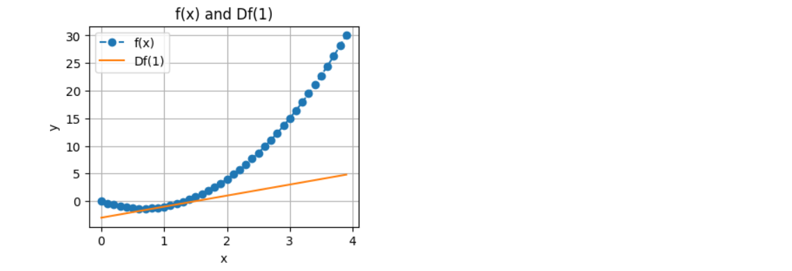
可视化

import matplotlib.pyplot as plt
import numpy as np
plt.figure(figsize=(4,3))
x=np.arange(0,4,0.1)
plt.xlabel("x")
plt.ylabel("y")
plt.title("f(x) and Df(1)")
plt.plot(x,f(x),'--o',label="f(x)")
plt.plot(x,2*x-3,'-',label="Df(1)")
plt.legend()
plt.grid()
plt.show()

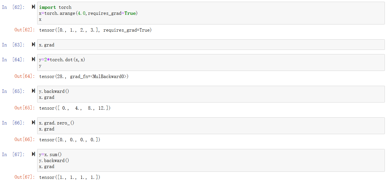
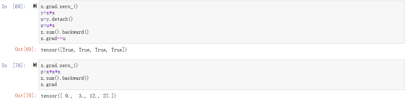
自动微分

非标量的反向传播

分离计算

概率

from torch.distributions import multinomial
import matplotlib.pyplot as plt
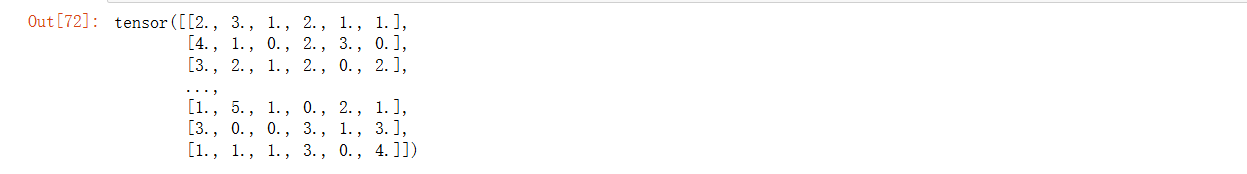
probs=torch.ones(6)/6
counts=multinomial.Multinomial(10,probs).sample((500,))
counts

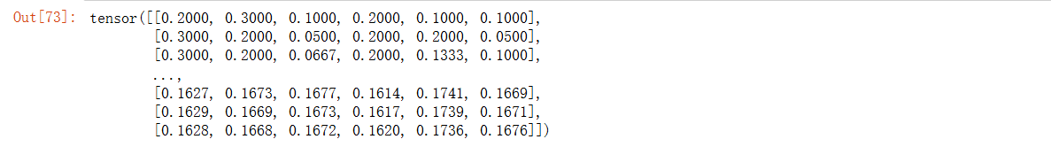
sum_cumsum=counts.cumsum(dim=0)
estimated=sum_cumsum/sum_cumsum.sum(dim=1,keepdims=True)
estimated

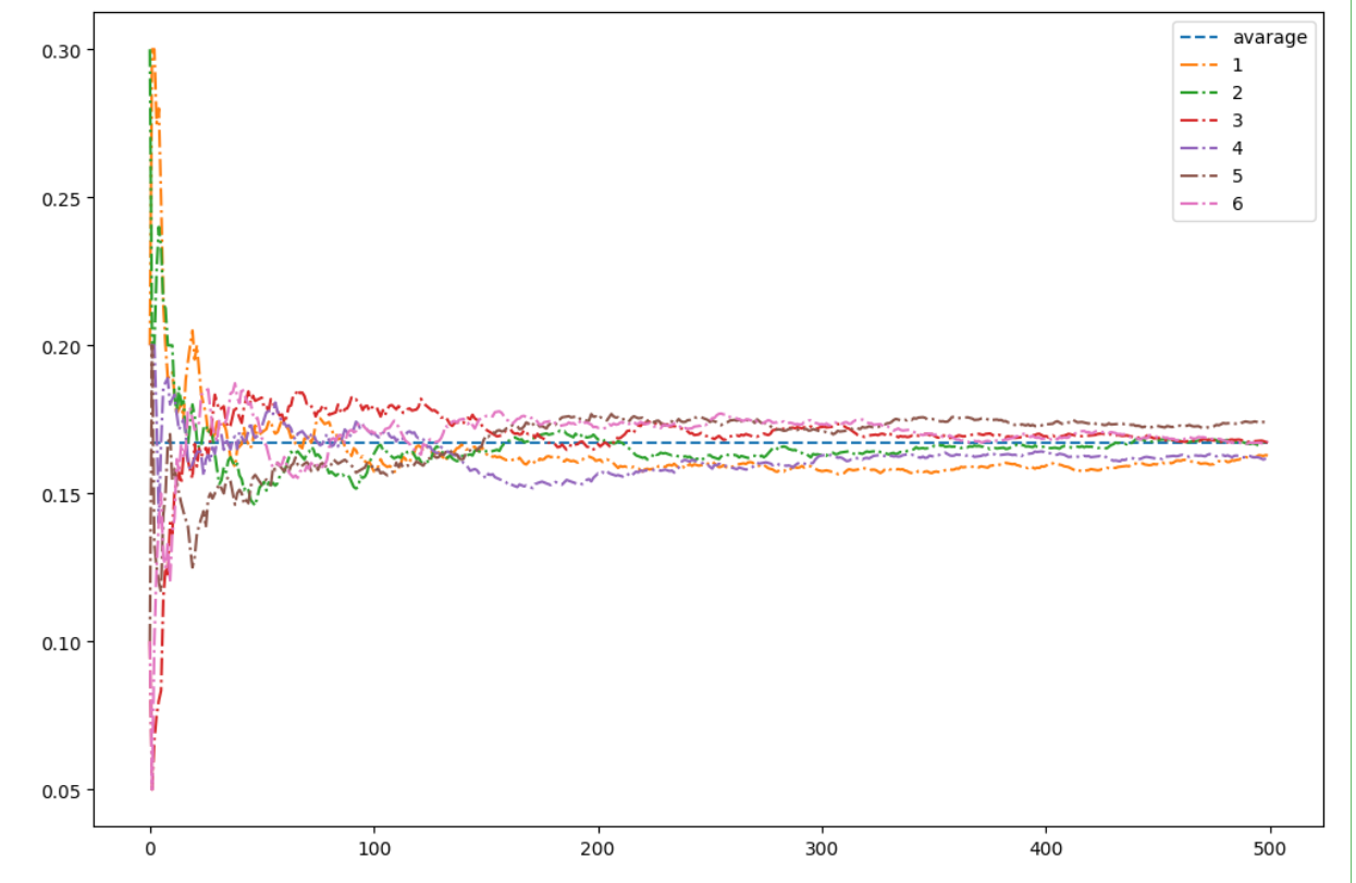
plt.figure(figsize=(12,8))
x=torch.arange(500)
y = torch.zeros(500) 
y[:]=0.167
plt.plot(x,y,'--',label="avarage")
for i in range(6):
    plt.plot(x,estimated[:,i],'-.',label=f"{i+1}")
plt.legend()
plt.show()

总结

这次学习也希望自己对于api的使用更加熟悉，而不是完全依赖ai，有些太新的东西，ai写的正确率也低一些。