谱聚类（spectral clustering)及其实现详解

Preface开了很多题，手稿都是写好一直思考如何放到CSDN上来，一方面由于公司技术隐私，一方面由于面向对象不同，要大改，所以一直没贴出完整，希望日后可以把开的题都补充全。谱聚类从构造规则化的拉普拉斯矩阵，到对特征矩阵的聚类，个中原理虽然简洁明了，但却蕴含了强大的逻辑结构。

杨铖

71329人浏览 · 2016-11-01 16:19:52

杨铖 · 2016-11-01 16:19:52 发布

Preface
开了很多题，手稿都是写好一直思考如何放到CSDN上来，一方面由于公司技术隐私，一方面由于面向对象不同，要大改，所以一直没贴出完整，希望日后可以把开的题都补充全。

先把大纲列出来：

一、从狄多公主圈地传说说起
二、谱聚类的演算
  （一）、演算
      1、谱聚类的概览
      2、谱聚类构图
      3、谱聚类切图
        （1）、RatioCut
        （2）、Ncut
        （3）、一点题外话
  （二）、pseudo-code
三、谱聚类的实现(scala)
  （一）、Similarity Matrix
  （二）、kNN/mutual kNN
  （三）、Laplacian Matrix
  （四）、Normalized
  （五）、Eigenvector(Jacobi methond)
  （六）、kmeans/GMM
四、一些参考文献

一、从狄多公主圈地传说说起

       谱聚类（spectral clustering）的思想最早可以追溯到一个古老的希腊传说，话说当时有一个公主，由于其父王去世后，长兄上位，想独揽大权，便杀害了她的丈夫，而为逃命，公主来到了一个部落，想与当地的酋长买一块地，于是将身上的金银财宝与酋长换了一块牛皮，且与酋长约定只要这块牛皮所占之地即可。聪明的酋长觉得这买卖可行，于是乎便答应了。殊不知，公主把牛皮撕成一条条，沿着海岸线，足足围出了一个城市。
       故事到这里就结束了，但是我们要说的才刚刚开始，狄多公主圈地传说，是目前知道的最早涉及Isoperimetric problem（等周长问题）的，具体为如何在给定长度的线条下围出一个最大的面积，也可理解为，在给定面积下如何使用更短的线条，而这，也正是谱图聚类想法的端倪，如何在给定一张图，拿出“更短”的边来将其“更好”地切分。而这个“更短”的边，正是对应了spectral clustering中的极小化问题，“更好”地切分，则是对应了spectral clustering中的簇聚类效果。
       谱聚类最早于1973年被提出，当时Donath 和 Hoffman第一次提出利用特征向量来解决谱聚类中的f向量选取问题，而同年，Fieder发现利用倒数第二小的特征向量，显然更加符合f向量的选取，同比之下，Fieder当时发表的东西更受大家认可，因为其很好地解决了谱聚类极小化问题里的NP-hard问题，这是不可估量的成就，虽然后来有研究发现，这种方法带来的误差，也是无法估量的，下图是Fielder老爷子，于去年15年离世，缅怀。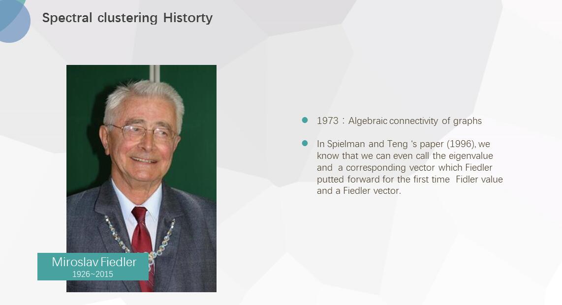

二、谱聚类的演算

（一）、演算

1、谱聚类概览

谱聚类演化于图论，后由于其表现出优秀的性能被广泛应用于聚类中，对比其他无监督聚类（如kmeans），spectral clustering的优点主要有以下：

1.过程对数据结构并没有太多的假设要求，如kmeans则要求数据为凸集。
2.可以通过构造稀疏similarity graph，使得对于更大的数据集表现出明显优于其他算法的计算速度。
3.由于spectral clustering是对图切割处理，不会存在像kmesns聚类时将离散的小簇聚合在一起的情况。
4.无需像GMM一样对数据的概率分布做假设。

同样，spectral clustering也有自己的缺点，主要存在于构图步骤，有如下：

1.对于选择不同的similarity graph比较敏感（如 epsilon-neighborhood， k-nearest neighborhood，fully connected等）。
2.对于参数的选择也比较敏感（如 epsilon-neighborhood的epsilon，k-nearest neighborhood的k，fully connected的 ）。

       谱聚类过程主要有两步，第一步是构图，将采样点数据构造成一张网图，表示为G(V,E)，V表示图中的点，E表示点与点之间的边，如下图：

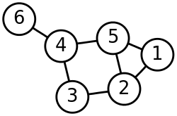
                            图1 谱聚类构图(来源wiki)
       第二步是切图，即将第一步构造出来的按照一定的切边准则，切分成不同的图，而不同的子图，即我们对应的聚类结果，举例如下：
               切图4
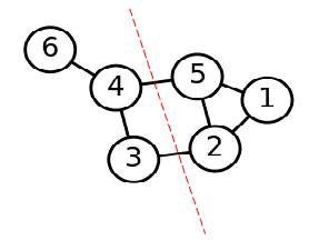
                            图2 谱聚类切图
       初看似乎并不难，但是…，下面详细说明推导。

2、谱聚类构图

       在构图中，一般有三种构图方式：
       1. ε <script type="math/tex" id="MathJax-Element-1">\varepsilon </script>-neighborhood
       2. k-nearest neighborhood
       3. fully connected
       前两种可以构造出稀疏矩阵，适合大样本的项目，第三种则相反，在大样本中其迭代速度会受到影响制约，在讲解三种构图方式前，需要引入similarity function，即计算两个样本点的距离，一般用欧氏距离： si,j=∥∥xi−xj∥∥2 <script type="math/tex" id="MathJax-Element-2">s_{i,j} = \left \| x_{i}-x_{j} \right \| ^{2} </script>, si,j <script type="math/tex" id="MathJax-Element-3">s_{i,j}</script>表示样本点 xi <script type="math/tex" id="MathJax-Element-4">x_{i}</script>与 xj <script type="math/tex" id="MathJax-Element-5">x_{j}</script>的距离，或者使用高斯距离 si,j=e−∥∥xi−xj∥∥22σ2 <script type="math/tex" id="MathJax-Element-6">s_{i,j}=e^{\frac{-\left \| x_{i}-x_{j} \right \|^{2}}{2\sigma ^{2}}}</script>，其中 σ <script type="math/tex" id="MathJax-Element-7">\sigma</script> 的选取也是对结果有一定影响，其表示为数据分布的分散程度，通过上述两种方式之一即可初步构造矩阵 S:Si,j=[s]i,j <script type="math/tex" id="MathJax-Element-8">S:S_{i,j}=[s]_{i,j}</script>，一般称为Similarity matrix(相似矩阵)。
       对于第一种构图 ε <script type="math/tex" id="MathJax-Element-9">\varepsilon</script> -neighborhood，顾名思义是取 si,j≤ε <script type="math/tex" id="MathJax-Element-10">s_{i,j}\leq \varepsilon</script>的点，则相似矩阵 S <script type="math/tex" id="MathJax-Element-11">S</script>可以进一步重构为邻接矩阵(adjacency matrix)W<script type="math/tex" id="MathJax-Element-12">W</script> :

W i, j = {0, i f s i, j > ε ε, i f s i, j \leq ε

ε <script type="math/tex" id="MathJax-Element-14">\varepsilon</script>-neighborhood重构下，样本点之间的权重没有包含更多的信息了。
对于第二种构图k-nearest neighborhood，其利用KNN算法，遍历所有的样本点，取每个样本最近的k个点作为近邻，但是这种方法会造成重构之后的邻接矩阵

W <script type="math/tex" id="MathJax-Element-15">W</script>非对称，为克服这种问题，一般采取下面两种方法之一：
一是只要点

xi<script type="math/tex" id="MathJax-Element-16">x_{i}</script>在

xj <script type="math/tex" id="MathJax-Element-17">x_{j}</script>的K个近邻中或者

xj <script type="math/tex" id="MathJax-Element-18">x_{j}</script>在

xi <script type="math/tex" id="MathJax-Element-19">x_{i}</script>的K个近邻中，则保留

si,j <script type="math/tex" id="MathJax-Element-20">s_{i,j}</script>，并对其做进一步处理

W <script type="math/tex" id="MathJax-Element-21">W</script>，此时为：

W i, j = W j, i = ⎧ ⎩ ⎨ 0, i f x i \notin K N N (X j) a n d x j \notin K N N (X i) e - ∥ ∥ x i - x j ∥ ∥ 2 2 σ 2, i f x i \in K N N (X j) o r x j \in K N N (X i)

si,j <script type="math/tex" id="MathJax-Element-23">s_{i,j}</script>并做进一步变换，此时

W <script type="math/tex" id="MathJax-Element-24">W</script>为：

W i, j = W j, i = ⎧ ⎩ ⎨ 0, i f x i \notin K N N (X j) o r x j \notin K N N (X i) e - ∥ ∥ x i - x j ∥ ∥ 2 2 σ 2, i f x i \in K N N (X j) a n d x j \in K N N (X i)

si,j=e−∥∥xi−xj∥∥22σ2 <script type="math/tex" id="MathJax-Element-26">s_{i,j}=e^{\frac{-\left \| x_{i}-x_{j} \right \|^{2}}{2\sigma ^{2}}}</script>，则重构之后的矩阵

W <script type="math/tex" id="MathJax-Element-27">W</script>与之前的相似矩阵

S<script type="math/tex" id="MathJax-Element-28">S</script>相同，为：

Wi,j=Si,j=[s]i,j <script type="math/tex" id="MathJax-Element-29">W_{i,j}= S_{i,j}=[s]_{i,j}</script>。
在了解三种构图方式后，还需要注意一些细节，对于第一二中构图，一般是重构基于欧氏距离的，而第三种构图方式，则是基于高斯距离的，注意到高斯距离的计算蕴含了这样一个情况：对于

∥∥xi−xj∥∥2 <script type="math/tex" id="MathJax-Element-30">\left \| x_{i}-x_{j} \right \|^{2}</script>比较大的样本点，其得到的高斯距离反而值是比较小的，而这也正是

S <script type="math/tex" id="MathJax-Element-31">S</script>可以直接作为

W<script type="math/tex" id="MathJax-Element-32">W</script>的原因，主要是为了将距离近的点的边赋予高权重。
得到邻接矩阵

W <script type="math/tex" id="MathJax-Element-33">W</script>后，需要做进一步的处理：
(1).计算阶矩(degree matrix)

D<script type="math/tex" id="MathJax-Element-34">D</script>：

D i, j = ⎧ ⎩ ⎨ ⎪ ⎪ 0, i f i \neq j \sum j w i, j, i f i = j

wi,j <script type="math/tex" id="MathJax-Element-36">w_{i,j}</script>为邻接矩阵

W <script type="math/tex" id="MathJax-Element-37">W</script>元素，

∑jwi,j<script type="math/tex" id="MathJax-Element-38">\sum_{j}w_{i,j}</script>表示将图中某点所连接的其他点的边的权重之和，可以看出，

D <script type="math/tex" id="MathJax-Element-39">D</script>为对角矩阵.
(2).计算拉普拉斯矩阵(Laplacians matrix)

L<script type="math/tex" id="MathJax-Element-40">L</script>：

L=D−W <script type="math/tex" id="MathJax-Element-41">L=D-W</script>
如此，在构图阶段基本就完成了，至于为什么要计算出拉普拉斯矩阵

L <script type="math/tex" id="MathJax-Element-42">L</script>，可以说

L=D−W<script type="math/tex" id="MathJax-Element-43">L=D-W</script>这种形式对于后面极大化问题是非常有利的(不知道前人是怎么想到的，不然

L <script type="math/tex" id="MathJax-Element-44">L</script>也不会被命名为拉普拉斯了吧)。

3、谱聚类切图

谱聚类切图存在两种主流的方式：RatioCut和Ncut，目的是找到一条权重最小，又能平衡切出子图大小的边，下面详细说明这两种切法。
在讲解RatioCut和Ncut之前，有必要说明一下问题背景和一些概念，假设V为所有样本点的集合，{A1,A2,⋯,Ak}<script type="math/tex" id="MathJax-Element-45">\{A_{1},A_{2},\cdots ,A_{k}\}</script>表示V的子集集合，其中 A1∪A2∪⋯∪Ak=V且A1∩A2∩⋯∩Ak=∅ <script type="math/tex" id="MathJax-Element-46">A_{1} \cup A_{2} \cup \cdots \cup A_{k}=V 且A_{1} \cap A_{2}\cap \cdots\cap A_{k}= \varnothing </script>，则子集与子集之间连边的权重和为：

c u t (A 1, A 2, \dots, A k) = 1 2 \sum i k W (A i, A i ¯)

Ai¯ <script type="math/tex" id="MathJax-Element-48">\bar{A_{i}}</script>为

Ai <script type="math/tex" id="MathJax-Element-49">A_{i}</script>的补集，意为除

Ai <script type="math/tex" id="MathJax-Element-50">A_{i}</script>子集外其他V的子集的并集，

W(Ai,Ai¯) <script type="math/tex" id="MathJax-Element-51">W(A_{i},\bar{A_{i}})</script>为

Ai <script type="math/tex" id="MathJax-Element-52">A_{i}</script>与其他子集的连边的和，为：

W (A i, A i ¯) = \sum m \in A i, n \in A i ¯ w m, n

wm,n <script type="math/tex" id="MathJax-Element-54">w_{m,n}</script>为邻接矩阵W中的元素。
由于我们切图的目的是使得每个子图内部结构相似，这个相似表现为连边的权重平均都较大，且互相连接，而每个子图间则尽量没有边相连，或者连边的权重很低，那么我们的目的可以表述为：

m i n c u t (A 1, A 2, \dots, A k)

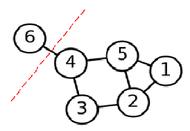
图3 问题切图
如上图，如果用

mincut(A1,A2,⋯,Ak) <script type="math/tex" id="MathJax-Element-56">min\quad cut(A_{1},A_{2},\cdots,A_{k})</script>这种方法切图，会造成将V切成很多个单点离散的图，显然这样是最快且最能满足那个最小化操作的，但这明显不是想要的结果，所以有了RatioCut和Ncut，具体地：

R a t i o c u t (A 1, A 2, \dots, A k) = 1 2 \sum i k W ( A i , A i ¯ ) | A i |

N c u t (A 1, A 2, \dots, A k) = 1 2 \sum i k W ( A i , A i ¯ ) v o l ( A i )

|Ai| <script type="math/tex" id="MathJax-Element-59">\left | A_{i} \right |</script> 为

Ai <script type="math/tex" id="MathJax-Element-60">A_{i}</script>中点的个数，

vol(Ai) <script type="math/tex" id="MathJax-Element-61">vol(A_{i})</script>为

Ai <script type="math/tex" id="MathJax-Element-62">A_{i}</script>中所有边的权重和。
下面详细讲解这两种方法的计算：Ratiocut & Ncut

(1).Ratiocut

Ratiocut切图考虑了目标子图的大小，避免了单个样本点作为一个簇的情况发生，平衡了各个子图的大小。Ratiocut的目标同样是极小化各子图连边和，如下：

m i n R a t i o c u t (A 1, A 2, \dots, A k)

{A1,A2,⋯,Ak} <script type="math/tex" id="MathJax-Element-64">\{A_{1},A_{2},\cdots ,A_{k}\}</script>的指示向量

hj={h1,h2,⋯,hi,⋯,hk},j=1,2,⋯,k <script type="math/tex" id="MathJax-Element-65">h_{j}=\{h_{1},h_{2},\cdots,h_{i},\cdots ,h_{k}\},\quad j=1,2,\cdots,k</script>. 其中i表示样本下标，j表示子集下标，表示样本i对子集j的指示，具体为：

h j, i = ⎧ ⎩ ⎨ ⎪ ⎪ ⎪ ⎪ 1 ∣ ∣ A j ∣ ∣ - - - \sqrt, i f v i \in A j 0, i f v i \notin A j

Aj <script type="math/tex" id="MathJax-Element-67">A_{j}</script>对应一个指示向量

hj <script type="math/tex" id="MathJax-Element-68">h_{j}</script>，而每个

hj <script type="math/tex" id="MathJax-Element-69">h_{j}</script>里有N个元素，分别代表N个样本点的指示结果，如果在原始数据中第i个样本被分割到子集

Aj <script type="math/tex" id="MathJax-Element-70">A_{j}</script>里，则

hj <script type="math/tex" id="MathJax-Element-71">h_{j}</script>的第i个元素为

1∣∣Aj∣∣√ <script type="math/tex" id="MathJax-Element-72">\frac{1}{\sqrt{\left | A_{j} \right |}}</script>，否则为0。
进一步，计算，可以得到：

h T i L h i = h T i (D - W) h i = h T i D h i - h T i W h i = \sum m = 1 \sum n = 1 h i, m h i, n D m, n - \sum m = 1 \sum n = 1 h i, m h i, n w m, n = \sum m = 1 h 2 i, m D m, m - \sum m = 1 \sum n = 1 h i, m h i, n w m, n = 1 2 (\sum m = 1 h 2 i, m D m, m - 2 \sum m = 1 \sum n = 1 h i, m h i, n w m, n + \sum n = 1 h 2 i, n D n, n)

hi <script type="math/tex" id="MathJax-Element-74">h_{i}</script>相乘有意义；
第五步，代数变换。
进一步地，做如下：

h T i L h i = 1 2 (\sum m = 1 h 2 i, m D m, m - 2 \sum m = 1 \sum n = 1 h i, m h i, n w m, n + \sum n = 1 h 2 i, n D n, n) = 1 2 (\sum m = 1 \sum n = 1 h 2 i, m w m, n - 2 \sum m = 1 \sum n = 1 h i, m h i, n w m, n + \sum n = 1 \sum m = 1 h 2 i, n w n, m) = 1 2 \sum m = 1 \sum n = 1 w n, m (h i, m - h i, n) 2

Dm,m=∑n=1wm,n <script type="math/tex" id="MathJax-Element-76">D_{m,m}=\sum_{n=1}w_{m,n}</script>
第二部到第三步，二次函数变换；
进一步，将上文

hj,i <script type="math/tex" id="MathJax-Element-77">h_{j,i}</script>代入上式，最终可以得到：

h T i L h i = 1 2 \sum m = 1 \sum n = 1 w m, n (h i, m - h i, n) 2 = 1 2 (\sum m \in A i, n \in A i ¯ w m, n (1 | A i | - - - \sqrt - 0) 2 + \sum m \in A i ¯, n \in A i w m, n (0 - 1 | A i | - - - \sqrt) 2) = 1 2 (\sum m \in A i, n \in A i ¯ w m, n 1 | A i | + \sum m \in A i ¯, n \in A i w m, n 1 | A i |) = 1 2 (c u t (A i, A i ¯) 1 | A i | + c u t (A i ¯, A i) 1 | A i |) = c u t ( A i , A i ¯ ) | A i | = R a t i o c u t (A i, A i ¯)

hi,m <script type="math/tex" id="MathJax-Element-79">h_{i,m}</script>，

hi,n <script type="math/tex" id="MathJax-Element-80">h_{i,n}</script>对应

Ai <script type="math/tex" id="MathJax-Element-81">A_{i}</script>的元素分别代入；
第三，四，五步，分别做简单运算，以及将

∑m∈Ai,n∈Ai¯wm,n <script type="math/tex" id="MathJax-Element-82">\sum_{m\in A_{i},n \in \bar{A_{i}}}w_{m,n}</script>替换为

cut(Ai,Ai¯) <script type="math/tex" id="MathJax-Element-83">cut(A_{i},\bar{A_{i}})</script>；
可以看到，通过引入指示变量h，将L矩阵放缩到与Ratiocut等价，这无疑是在谱聚类中划时代的一举。
为了更进一步考虑进所有的指示向量，令

H={h1,h2,⋯,hk} <script type="math/tex" id="MathJax-Element-84">H=\{h_{1},h_{2},\cdots ,h_{k}\}</script>，其中

hi <script type="math/tex" id="MathJax-Element-85">h_{i}</script>按列排列，由

hi <script type="math/tex" id="MathJax-Element-86">h_{i}</script>的定义知每个

hi <script type="math/tex" id="MathJax-Element-87">h_{i}</script>之间都是相互正交，即

hi∗hj=0,i≠j <script type="math/tex" id="MathJax-Element-88">h_{i}*h_{j}=0,i \neq j</script>，且有

hi∗hi=1 <script type="math/tex" id="MathJax-Element-89">h_{i}*h_{i}=1</script>，可得到：

R a t i o c u t (A 1, A 2, \dots, A k) = \sum i = 1 k h T i L h i = \sum i = 1 k (H T L H) i i = T r (H T L H)

minRatiocut(A1,A2,⋯,Ak) <script type="math/tex" id="MathJax-Element-91">min\quad Ratiocut(A_{1},A_{2},\cdots,A_{k})</script>，转化为：

a r g m i n H T r (H T L H), s . t . H T H = I

Tr(HTLH) <script type="math/tex" id="MathJax-Element-93">Tr(H^{T}LH)</script>最小。
注意到一点，要求条件下的H，首先是求得组成H的每个

hi <script type="math/tex" id="MathJax-Element-94">h_{i}</script>，而每个

hi <script type="math/tex" id="MathJax-Element-95">h_{i}</script>都是Nx1的向量，且向量中每个值都是二值分布，即取值0或者

1/|Ai|−−−√ <script type="math/tex" id="MathJax-Element-96">1/\sqrt{\left | A_{i} \right |}</script>，那么对于每个元素，有2种选择，则当个

hi <script type="math/tex" id="MathJax-Element-97">h_{i}</script>就有

2N <script type="math/tex" id="MathJax-Element-98">2^{N}</script>种情况，对于整个H矩阵，则有

(C1k)N <script type="math/tex" id="MathJax-Element-99">(C_{k}^{1})^{N}</script>种情况，对于N很大的数据，这无疑是灾难性的NP-hard问题，显然我们不可能遍历所有的情况来求解，那么问题是不是没有解？答案自然是否定的，虽然我们没办法求出精确的，但是我们可以用另外一种方法近似代替

hi <script type="math/tex" id="MathJax-Element-100">h_{i}</script>，而这就是文章开头Fielder提出来的，当k=2的时候，可以用L的倒数第二小的特征向量(因为最小的特征向量为1，其对应的特征值为0，不适合用来求解)来代替，关于具体为什么可以这么做，可以参考Rayleigh-Ritz method(对应论文为：A short theory of the Rayleigh-Ritz method)，因为涉及泛函变分，这里就不多说了。
那么当k取任意数字时，只需取L矩阵对应的最小那k个（毕竟倒数第二小只有1个），即可组成目标H，最后，对H做标准化处理，如下：

H * i, j = H i , j ( \sum k j = 1 H 2 i , j ) 1 / 2

Tr(HTLH) <script type="math/tex" id="MathJax-Element-102"> Tr(H^{T}LH)</script>的最小值是多少，而是求能最小化

Tr(HTLH) <script type="math/tex" id="MathJax-Element-103"> Tr(H^{T}LH)</script>的H，所以聚类的时候，分别对H中的行进行聚类即可，通常是kmeans，也可以是GMM，具体看效果而定。
       至于为什么是对H的行进行聚类，有两点原因：
       1.注意到H除了是能满足极小化条件的解，还是L的特征向量，也可以理解为W的特征向量，而W则是我们构造出的图，对该图的特征向量做聚类，一方面聚类时不会丢失原图太多信息，另一方面是降维加快计算速度，而且容易发现图背后的模式。
       2.由于之前定义的指示向量

hi <script type="math/tex" id="MathJax-Element-104">h_{i}</script>是二值分布，但是由于NP-hard问题的存在导致

hi <script type="math/tex" id="MathJax-Element-105">h_{i}</script>无法显式求解，只能利用特征向量进行近似逼近，但是特征向量是取任意值，结果是我们对

hi <script type="math/tex" id="MathJax-Element-106">h_{i}</script>的二值分布限制进行放松，但这样一来

hi <script type="math/tex" id="MathJax-Element-107">h_{i}</script>如何指示各样本的所属情况？所以kmeans就登场了，利用kmeans对该向量进行聚类，如果是k=2的情况，那么kmeans结果就与之前二值分布的想法相同了，所以kmeans的意义在此，k等于任意数值的情况做进一步类推即可。
以上是Ratiocut的内容。

(2).Ncut

Ncut切法实际上与Ratiocut相似，但Ncut把Ratiocut的分母 |Ai| <script type="math/tex" id="MathJax-Element-108">|A_{i}|</script>换成 vol(Ai) <script type="math/tex" id="MathJax-Element-109">vol(A_{i})</script> ，这种改变与之而来的，是L的normalized，这种特殊称谓会在下文说明，而且这种normalized，使得Ncut对于spectral clustering来说，其实更好，下文会说明。
同样，Ncut的目标，也是极小化各子图连边的和，如下：

m i n N c u t (A 1, A 2, \dots, A k)

{A1,A2,⋯,Ak} <script type="math/tex" id="MathJax-Element-111">\{A_{1},A_{2},\cdots ,A_{k}\}</script>的指示变量

hj={h1,h2,⋯,hi,⋯,hk},j=1,2,⋯,k <script type="math/tex" id="MathJax-Element-112">h_{j}=\{h_{1},h_{2},\cdots,h_{i},\cdots ,h_{k}\},\quad j=1,2,\cdots,k</script>，同样，其中i表示样本下标，j表示子集下标，

hj,i <script type="math/tex" id="MathJax-Element-113">h_{j,i}</script>表示样本i对子集j的指示，不同的是，其具体为：

h j, i = ⎧ ⎩ ⎨ ⎪ ⎪ 1 v o l ( A i ) - - - - - - \sqrt, i f v i \in A j 0, i f v i \notin A j

Aj <script type="math/tex" id="MathJax-Element-115">A_{j}</script>里，则

hj <script type="math/tex" id="MathJax-Element-116">h_{j}</script>的第i个元素为

1/vol(Ai)−−−−−−√ <script type="math/tex" id="MathJax-Element-117">1/\sqrt{vol(A_{i})}</script>，否则为0。
进一步，计算

hTiLhi <script type="math/tex" id="MathJax-Element-118">h_{i}^{T}Lh_{i} </script>，可以得到：

h T i L h i = h T i D h i - h T i W h i = \sum m = 1 \sum n = 1 h i, m h i, n D m, n - \sum m = 1 \sum n = 1 h i, m h i, n w m, n = \sum m = 1 h 2 i, m D m, m - \sum m = 1 \sum n = 1 h i, m h i, n w m, n = 1 2 (\sum m = 1 h 2 i, m D m, m - 2 \sum m = 1 \sum n = 1 h i, m h i, n w m, n + \sum n = 1 h 2 i, n D n, n) = 1 2 (\sum m = 1 \sum n = 1 h 2 i, m w m, n - 2 \sum m = 1 \sum n = 1 h i, m h i, n w m, n + \sum n = 1 \sum m = 1 h 2 i, n w n, m) = 1 2 \sum m = 1 \sum n = 1 w m, n (h i, m - h i, n) 2 = 1 2 (\sum m \in A i, n \in A i ¯ w m, n (1 v o l ( A i ) - - - - - - \sqrt - 0) 2 + \sum m \in A i ¯, n \in A i w m, n (0 - 1 v o l ( A i ) - - - - - - \sqrt) 2) = c u t ( A i , A i ¯ ) v o l ( A i ) = N c u t (A i, A i ¯)

hTiLhi <script type="math/tex" id="MathJax-Element-120">h_{i}^{T}Lh_{i}</script>如何得到

Ncut(Ai,Ai¯) <script type="math/tex" id="MathJax-Element-121">Ncut(A_{i},\bar{A_{i}})</script>，以便将

minNcut(A1,A2,⋯,Ak) <script type="math/tex" id="MathJax-Element-122">min\quad Ncut(A_{1},A_{2},\cdots,A_{k})</script>用严谨数学式子进行表达。
       这里对上述一大串式子分解一下：
       第一，二，三步，做一些简单的变换，如L=D-W代入，将向量内积转换成连加形式，同样，D是对角矩阵，可省去一些项；
       第四，五，六步，主要是做二次函数变换；
       第七步，将

hi,m <script type="math/tex" id="MathJax-Element-123">h_{i,m}</script>，

hi,n <script type="math/tex" id="MathJax-Element-124">h_{i,n}</script>对应

Ai <script type="math/tex" id="MathJax-Element-125">A_{i}</script>的元素分别代入；
第八，九步，得到

Ncut(Ai,Ai¯) <script type="math/tex" id="MathJax-Element-126">Ncut(A_{i},\bar{A_{i}})</script> 形式；
此外，相比与Ratiocut，Ncut特有的一点性质是：

hTiDhi=1 <script type="math/tex" id="MathJax-Element-127"> h_{i}^{T}Dh_{i}=1</script>，具体如下：

h T i D h i = \sum n = 1 h 2 i, n D n, n = \sum v n \in A i 1 v o l ( A i ) D n, n + \sum v n \notin A i 0 \cdot D n, n = 1 v o l ( A i ) \sum v n \in A i w v n + 0 = 1 v o l ( A i ) v o l (A i) = 1

H={h1,h2,⋯,hk} <script type="math/tex" id="MathJax-Element-129">H=\{h_{1},h_{2},\cdots ,h_{k}\}</script>，则

HTDH=I <script type="math/tex" id="MathJax-Element-130">H^{T}DH=I</script> ,其中I为单位对角矩阵。
同样，可以得到：

N c u t (A 1, A 2, \dots, A k) = \sum i = 1 k h T i L h i = \sum i = 1 k (H T L H) i i = T r (H T L H)

minNcut(A1,A2,⋯,Ak) <script type="math/tex" id="MathJax-Element-132">min\quad Ncut(A_{1},A_{2},\cdots,A_{k})</script>，转化为：

a r g m i n H T r (H T L H), s . t . H T D H = I

H=D−1/2F <script type="math/tex" id="MathJax-Element-134">H=D^{-1/2}F</script>，

D−1/2 <script type="math/tex" id="MathJax-Element-135">D^{-1/2}</script>意为对D对角线上元素开方再求逆。将

H=D−1/2F <script type="math/tex" id="MathJax-Element-136">H=D^{-1/2}F</script>代入

argminHTr(HTLH),s.t.HTDH=I <script type="math/tex" id="MathJax-Element-137"> arg\mathop{min}\limits_{H} \quad Tr(H^{T}LH), \quad s.t. H^{T}DH=I</script>，可以得到：

H T L H = (D - 1 / 2 F) T L D - 1 / 2 F = F T D - 1 / 2 L D - 1 / 2 F

H T D H = (D - 1 / 2 F) T D D - 1 / 2 F = F T D - 1 / 2 L D - 1 / 2 F = F T I F = I

argminHTr(HTLH),s.t.HTDH=I <script type="math/tex" id="MathJax-Element-140"> arg\mathop{min}\limits_{H} \quad Tr(H^{T}LH), \quad s.t. H^{T}DH=I</script>可以修改为：

a r g m i n H T r (F T D - 1 / 2 L D - 1 / 2 F), s . t . F T F = I

D−1/2LD−1/2 <script type="math/tex" id="MathJax-Element-142">D^{-1/2}LD^{-1/2}</script>这一步操作，就是对L矩阵进行normalize，而normalize可以理解为标准化，具体为：

Li,jvol(Ai)vol(Aj)√ <script type="math/tex" id="MathJax-Element-143">\frac{L_{i,j}}{\sqrt{vol( A_{i})vol(A_{j})}}</script> ，这么做的一个好处就是对L中的元素进行标准化处理使得不同元素的量纲得到归一，具体理解就是，同个子集里，不同样本点之间的连边可能大小比较相似，这点没问题，但是对于不同子集，样本点之间的连边大小可能会差异很大，做这一步normalize操作，可以将L中的元素归一化在[-1,1]之间，这样量纲一致，对算法迭代速度，结果的精度都是有很大提升。
最后，F矩阵的求解可通过求

D−1/2LD−1/2 <script type="math/tex" id="MathJax-Element-144">D^{-1/2}LD^{-1/2}</script>的前k个特征向量组成，然后对F再做进一步的标准化：

F * i, j = F i , j ( \sum k j = 1 F 2 i , j ) 1 / 2

(3).一点题外话

       写到这里，如果只是应用spectral clustering，则此部分可以忽略，直接看下文pseudo-code部分即可，但是对于喜欢深入探究，不妨看一看。
       值得一提的是，从概率的视角出发，与上文推导也是不谋而合，而且得到的结论，与Ncut更是异曲同工。这种概率视角在多数论文里，称之为随机游走(Random walks)，在随机数学里，常见于马尔可夫模型。这部分的详细出处可以参考Lovaszl(1993: Random Walks on Graphs: A Survey)，以及Meila & Shi (2001:A Random Walks Views of Spectral Segmentation)。
       在随机游走框架下，通常都会构建一个转移概率矩阵(transition matrix)，同样，利用上文的邻接矩阵，可以得到该转移概率矩阵P为：

P i, j = w i, j / D i, j, i, j = 1, 2, \dots, N

wi,j <script type="math/tex" id="MathJax-Element-147">w_{i,j}</script>，

Di,j <script type="math/tex" id="MathJax-Element-148">D_{i,j}</script> 分别为W，D矩阵中的元素。可以看出，其实

P=WD−1 <script type="math/tex" id="MathJax-Element-149">P=WD^{-1}</script>。为方便做进一步论述，假设一个初始分布概率

π=(π1,π2,⋯,πi,⋯,πN)T <script type="math/tex" id="MathJax-Element-150">\pi = (\pi_{1},\pi_{2},\cdots,\pi_{i},\cdots,\pi_{N})^{T}</script>，其中：

π i = D i , i v o l ( V )

A1 <script type="math/tex" id="MathJax-Element-152">A_{1}</script>以及

A2 <script type="math/tex" id="MathJax-Element-153">A_{2}</script>，则目标是极小化下面概率：

m i n 1 2 (P (A 1 | A 2) + P (A 2 | A 1))

P(A1|A2) <script type="math/tex" id="MathJax-Element-155">P(A_{1}|A_{2})</script>，可以写为：

P (A 1 | A 2) = P ( A 1 , A 2 P ( A 2 )

P(A2) <script type="math/tex" id="MathJax-Element-157">P(A_{2})</script>，可以理解为任意样本属于

A2 <script type="math/tex" id="MathJax-Element-158">A_{2}</script>的概率，则：

P (A 2) = v o l ( A 2 ) v o l ( A )

A2 <script type="math/tex" id="MathJax-Element-160">A_{2}</script>簇里边和与整张图V边和做对比。
对于

P(A1,A2) <script type="math/tex" id="MathJax-Element-161">P(A_{1},A_{2})</script>，可以理解为，任取一点，其从

A2 <script type="math/tex" id="MathJax-Element-162">A_{2}</script>切换至

A1 <script type="math/tex" id="MathJax-Element-163">A_{1}</script>的概率，具体为：

P (A 1, A 2) = \sum i \in A 1, j \in A 2 π i P i, j = \sum i \in A 1, j \in A 2 D i , j v o l ( V ) w i , j D i , j = 1 v o l ( V ) \sum i \in A 1, j \in A 2 w i, j

P (A 1 | A 2) = 1 v o l ( V ) \sum i \in A 1 , j \in A 2 w i , j v o l ( A 2 ) v o l ( V ) = \sum i \in A 1 , j \in A 2 w i , j v o l ( A 2 )

m i n 1 2 (P (A 1 | A 2) + P (A 2 | A 1)) = m i n 1 2 (\sum i \in A 1 , j \in A 2 w i , j v o l ( A 2 ) + \sum i \in A 1 , j \in A 2 w i , j v o l ( A 1 )) = m i n 1 2 \sum i = 1 2 W ( A i , A i ¯ ) v o l ( A i )

（二）、pesudo-code

       Spectral clustering的pseudo-code有很多种，这里只讲最常用的normalized版本，也就是Ncut作为切图法的版本。
       具体为：
       1.构造S矩阵(similarity matrix)，同时指定要聚类的簇数k；
       2.利用S矩阵构造W矩阵(adjacent matrix)；
       3.计算拉普拉斯矩阵L，其中L=D-W；
       4.对L矩阵标准化，即令；
       5.计算normalize后的L矩阵的前k个特征向量，按特征值升序排列；
       6.对k个向量组成的矩阵的行进行看kmeans/GMM聚类；
       7.将聚类结果的各个簇分别打上标记，对应上原数据，输出结果。

input: (data,K,k,kNNType,sigma,epsilon)
1. S = Euclidean(data) 
2. W = Gaussian( kNN(S,k,kNNType) , sigma ) 
3. L = D - W
4. L' = normalized(L)
5. EV = eigenvector(L',K)
6. while( (newCenter - oldCenter) > epsilon){
      newCenter = kmeans(EV,K)
   }
output：K clusters of SC

其中，data为样本，对应code为二维数组，K为要聚类的簇数，k为kNN的邻接个数，kNNType为SC中的kNN函数类型，一般为kNN/mutalkNN，具体看上文说明，sigma为构造W矩阵时的高斯函数参数，epsilon为kmeans或者GMMs中的更新步长。SC输出为聚出K个簇。

三、谱聚类的实现

实现过程涉及到的一些概念有：Similarity Matrix、kNN/mutual kNN、Laplacian Matrix、Normalized、Eigenvector(Jacobi methond)、kmeans/GMM；下面一一按序解析，使用语言为scala，这里需要说明一点，由于技术保密，这里有些东西只能介绍一些简单的版本，动手操作可以发现，上述计算在小样本还算过得去，样本一大简直无法入目，只能各位自己多去查看论文了，若日后有缘，会开篇做另外的优化阐述。

（一）、Similarity Matrix

// calculate the similarity matrix
def calculateSimilarityMatrix(SCInput: Array[Array[Double]]): Array[Array[Double]] = {
    // the Euclidean Distance
    def SCEuclideanDistance(SCEDInput: Array[Double]): Array[Double] = {
        SCInput.map(_.zip(SCEDInput))
               .map(a => a.map(b => math.pow(b._1 - b._2, 2)).sum)
     }
     SCInput.map(SCEuclideanDistance)
}

       这里不代入数据了，直接构造一个similarity Matrix了，如下：

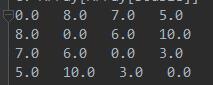
                     图4 similarity Matrix

（二）、kNN/mutual kNN

下面是对上面similarity matrix一步构造的相似图做调整，将其转化为W（adjacency matrix）.

    // define the kNN function
    def kNN(k: Int, kNNType: String, sigma: Double = 1.0, SMatrix: Array[Array[Double]]): Array[Array[Double]] = {
        val len = SMatrix.length
        val AdjacencyMatrix = Array.ofDim[Double](len, len)

        // define the function of calculating the mutual adjacency matrix (for mutualkNN)
        @tailrec
        def calculateMutualAdjacencyMatrix(n: Int, S: Array[Array[Double]]): Array[Array[Double]] = {
            if (n < len) {
                // take out the smallest k values
                val kSmallestValue = S(n).zipWithIndex.sortWith((a, b) => a._1 < b._1).take(k + 1)
                val indexOfValue = kSmallestValue.map(_._2).distinct
                // calculate the Gaussian similarity value
                for (i <- indexOfValue) {
                    val GaussianSimilarity = math.exp(-S(n)(i) / 2 / sigma / sigma)
                    AdjacencyMatrix(n)(i) = GaussianSimilarity
                }
                calculateMutualAdjacencyMatrix(n + 1, S)
            } else {
                // judge mutual or not.
                for (i <- 0 until len) {
                    val notZero = AdjacencyMatrix(i).zipWithIndex.filter(_._1 != 0.0).map(_._2)
                    for (j <- notZero) if (AdjacencyMatrix(j)(i) == 0.0) AdjacencyMatrix(i)(j) = 0.0
                }
                AdjacencyMatrix
            }
        }

        // define the function of calculating the mutual adjacency matrix (for kNN)
        @tailrec
        def calculateAdjacencyMatrix(n: Int, S: Array[Array[Double]]): Array[Array[Double]] = {
            if (n < len) {
                // take out the smallest k values
                val kSmallestValue = S(n).zipWithIndex.sortWith((a, b) => a._1 < b._1).take(k + 1)
                val indexOfValue = kSmallestValue.map(_._2).distinct
                // calculate the Gaussian similarity value
                for (i <- indexOfValue) {
                    val GaussianSimilarity = math.exp(-S(n)(i) / 2 / sigma / sigma)
                    AdjacencyMatrix(n)(i) = GaussianSimilarity
                    AdjacencyMatrix(i)(n) = GaussianSimilarity
                }
                calculateAdjacencyMatrix(n + 1, S)
            } else {
                AdjacencyMatrix
            }
        }

        if (kNNType == "mutualkNN") {
            calculateMutualAdjacencyMatrix(0, SMatrix)
        } else {
            calculateAdjacencyMatrix(0, SMatrix)
        }
    }

       两种操作结果如下：kNN和mutualkNN。PS：由于是直接在IntelliJ直接截图，所以看起来可能没那么好看(ㄒoㄒ)
               kNN
                     图5 adjacency Matrix (kNN)

图6 adjacency Matrix (mutualkNN)

两个矩阵计算时k值均指定为2，sigma指定为1，可以观察出，上文矩阵 ⎡⎣⎢⎢⎢0.08.07.05.08.00.06.010.07.06.00.03.05.010.03.00.0⎤⎦⎥⎥⎥ <script type="math/tex" id="MathJax-Element-167"> \begin{bmatrix} 0.0 & 8.0 & 7.0 & 5.0 \\ 8.0 & 0.0 & 6.0 & 10.0 \\ 7.0 & 6.0 & 0.0 & 3.0 \\ 5.0 & 10.0 & 3.0 & 0.0 \end{bmatrix}</script> ，其对应的kNN处理后的W矩阵，比较容易理解，即取任意样本最近的2个样本作为连点即可，而mutualkNN处理后的W矩阵，则需保证连点的两边均是该两点的最近的2个样本之一，举个例子，与第1个样本最近的两个点分别为第3，4个点，其距离分别为7.0和5.0，而第3个点最近的两个点分别为第2，4个点，其距离为6.0和3.0，所以这样下来，与第1个样本连边的点就只有第4个点，看图6可明白。

（三）、 Laplacian Matrix

下面利用上面W（adjacency matrix）矩阵，进一步计算D（degree matrix）矩阵和L（laplacian matrix）矩阵.

    // define the function of calculating the Laplacian Matrix
    def calculateLaplacianMatrix(adjacencyMatrix: Array[Array[Double]]): Array[Array[Double]] = {
        val len = adjacencyMatrix.length
        val laplacianMatrix = Array.ofDim[Double](len, len)

        // define the function of calculating the degree matrix
        def calculateDegreeMatrix(AM: Array[Array[Double]]): Array[Array[Double]] = {
            val degreeMatrix = Array.ofDim[Double](len, len)
            for (i <- 0 until len) {
                degreeMatrix(i)(i) = AM(i).sum
            }
            degreeMatrix
        }
        val degreeMatrix = calculateDegreeMatrix(adjacencyMatrix)

        // calculate the Laplacian matrix
        for (i <- 0 until len) {
            laplacianMatrix(i) = degreeMatrix(i).zip(adjacencyMatrix(i)).map(a => a._1 - a._2)
        }
        laplacianMatrix
    }

       这里我把D的计算和L的计算写在一起，一步计算到位，结果如下：
               degreeMatrix
                     图7 degree Matrix

laplacianMatrix
图8 laplacian Matrix

（四）、 Normalized

下面进一步对上面L（laplacian matrix）矩阵进行正则化处理.

    // define the function of calculating the normalized Laplacian Matrix
    def Normalized(laplacianMatrix: Array[Array[Double]], adjacencyMatrix: Array[Array[Double]]): Array[Array[Double]] = {
        val len = adjacencyMatrix.length

        // define the function of calculate the -1/2 power of the degree matrix
        def calculateAdjustDegreeMatrix(AM: Array[Array[Double]]): Array[Array[Double]] = {
            val adjustDegreeMatrix = Array.ofDim[Double](len, len)
            for (i <- 0 until len) {
                adjustDegreeMatrix(i)(i) = 1 / math.pow(AM(i).sum, 0.5)
            }
            adjustDegreeMatrix
        }
        val adjustDegreeMatrix = calculateAdjustDegreeMatrix(adjacencyMatrix)

        // calculate the normalized laplacian matrix
        def matrixProduct(left: Array[Array[Double]], right: Array[Array[Double]]): Array[Array[Double]] = {
            val len = left.length
            val output = Array.ofDim[Double](len,len)

            for(i <- 0 until len; j <- i until len){
                output(i)(j) = left(i).zip(right.map(_(j))).map(a => a._1 * a._2).sum
                output(j)(i) = output(i)(j)
            }
            output
        }
        val temp = matrixProduct(adjustDegreeMatrix,laplacianMatrix)
        val normalizedLaplacianMatrix = matrixProduct(temp,adjustDegreeMatrix)
        normalizedLaplacianMatrix
    }

       下面是上文L（laplacian matrix）矩阵的正则结果：

                     图9 Normalized laplacian Matrix

（五）、 Eigenvector(Jacobi methond)

下面进一步对上面正则化处理之后的L矩阵L’，取对应的特征向量，组成新的矩阵，特征向量的计算这里用的是串行的Jacobi旋转方法，内在逻辑就是对L’矩阵行列转换，得到L’的相似矩阵，且满足该相似矩阵为对角矩阵。值得一说的是，这种方法小样本可行，大样本效率很低，之后看情况，看是否再把优化的方法写出来，看缘分吧。。。

    // define the function of calculating the k smallest eigenvectors of normalized laplacian matrix with Jacobi method.
    def kSmallestEigenvectors(k: Int, normalizedLaplacian: Array[Array[Double]]): (Array[Double], Array[Array[Double]]) = {

        val len = normalizedLaplacian.length

        // initial the eigenvector matrix.
        val eigenvectorMatrix = Array.ofDim[Double](len, len)
        for (i <- 0 until len) eigenvectorMatrix(i)(i) = 1.0

        // initial the parameter of epsilon.
        val epsilon = (math.pow(10, -10), -1)

        // calculate the largest one Of normalized laplacian matrix(off-diagonal).
        def calculateLargestOfNormL(Input: Array[Array[Double]]): (Double, Int) = {
            val temp = Input.map(_.zipWithIndex)
            val largestOfRow = new Array[(Double, Int)](len - 1)
            for (i <- 0 until (len - 1)) {
                largestOfRow(i) = temp(i).filter(_._2 > i).sortWith((a, b) => a._1.abs > b._1.abs).head
            }
            val largestOfInput = largestOfRow.sortWith((a, b) => a._1.abs > b._1.abs).head
            if (epsilon._1 > largestOfInput._1.abs) epsilon else largestOfInput
        }
        var largestOfNormL = calculateLargestOfNormL(normalizedLaplacian)

        // Judge condition.
        var loop: Boolean = true

        // main loop.
        while (loop) {

            // the index of the largest value of normalized laplacian matrix.
            val mRow = largestOfNormL._2
            val mCol = normalizedLaplacian(largestOfNormL._2).indexOf(largestOfNormL._1)

            // calculate the new normalized Laplacian matrix: angle, sin, cos, new(row,col)
            // cache the temp value.
            val nL_ij = normalizedLaplacian(mRow)(mCol)
            val nL_ii = normalizedLaplacian(mRow)(mRow)
            val nL_jj = normalizedLaplacian(mCol)(mCol)
            val angle = if (nL_jj == nL_ii) math.Pi / 4.0 else 0.5 * math.atan2(2 * nL_ij, nL_jj - nL_ii)
            val sinAngle = math.sin(angle)
            val cosAngle = math.cos(angle)
            // update the normalized Laplacian matrix (ii, jj, ij, ji)
            normalizedLaplacian(mRow)(mRow) = nL_ii * cosAngle * cosAngle + nL_jj * sinAngle * sinAngle - 2 * nL_ij * cosAngle * sinAngle
            normalizedLaplacian(mCol)(mCol) = nL_ii * sinAngle * sinAngle + nL_jj * cosAngle * cosAngle + 2 * nL_ij * cosAngle * sinAngle
            normalizedLaplacian(mRow)(mCol) = (cosAngle * cosAngle - sinAngle * sinAngle) * nL_ij + sinAngle * cosAngle * (nL_ii - nL_jj)
            normalizedLaplacian(mCol)(mRow) = normalizedLaplacian(mRow)(mCol)
            for (i <- (0 until len).filter(a => a != mRow && a != mCol)) {
                val tempRi = normalizedLaplacian(mRow)(i)
                val tempCi = normalizedLaplacian(mCol)(i)
                normalizedLaplacian(mRow)(i) = cosAngle * tempRi - sinAngle * tempCi
                normalizedLaplacian(mCol)(i) = sinAngle * tempRi + cosAngle * tempCi
                normalizedLaplacian(i)(mRow) = normalizedLaplacian(mRow)(i)
                normalizedLaplacian(i)(mCol) = normalizedLaplacian(mCol)(i)
            }

            // update the eigenvector matrix.
            for (i <- 0 until len) {
                val eigenIR = eigenvectorMatrix(i)(mRow)
                val eigenIC = eigenvectorMatrix(i)(mCol)
                eigenvectorMatrix(i)(mRow) = eigenIR * cosAngle - eigenIC * sinAngle
                eigenvectorMatrix(i)(mCol) = eigenIC * cosAngle + eigenIR * sinAngle
            }

            // update the temp value again.
            largestOfNormL = calculateLargestOfNormL(normalizedLaplacian)

            // update the judge condition.
            if (largestOfNormL._2 == -1) loop = false

        }

        // return the k smallest eigenvalue and it's corresponding eigenvector matrix.
        val eigenvalue = new Array[Double](len)
        for (i <- 0 until len) eigenvalue(i) = normalizedLaplacian(i)(i)
        def kSmallest(eigenvalue: Array[Double], eigenvector: Array[Array[Double]]): (Array[Double], Array[Array[Double]]) = {
            val eigenvalueWithIndex = eigenvalue.zipWithIndex.sortWith((a, b) => a._1 < b._1).take(k)
            val ouput = Array.ofDim[Double](len, k)
            var n: Int = 0
            for ((v, i) <- eigenvalueWithIndex) {
                for (j <- 0 until len) {
                    ouput(j)(n) = eigenvector(j)(i)
                }
                n += 1
            }
            (eigenvalueWithIndex.map(_._1), ouput)
        }
        val kSmallestValueVector = kSmallest(eigenvalue, eigenvectorMatrix)

        // final ouput.
        (kSmallestValueVector._1, kSmallestValueVector._2)

    }

       为直观一点，下面拿矩阵 ⎡⎣⎢⎢⎢0.08.07.05.08.00.06.010.07.06.00.03.05.010.03.00.0⎤⎦⎥⎥⎥ <script type="math/tex" id="MathJax-Element-168"> \begin{bmatrix} 0.0 & 8.0 & 7.0 & 5.0 \\ 8.0 & 0.0 & 6.0 & 10.0 \\ 7.0 & 6.0 & 0.0 & 3.0 \\ 5.0 & 10.0 & 3.0 & 0.0 \end{bmatrix}</script> 计算特征值和特征向量，结果如下：

                     图10 特征值（对角线）

图11 特征向量

结果可以和Matlab和R，python做比较，我只和R比对过，基本无差。

（六）、 kmeans/GMM

再做一步最终的聚类，便基本完成了算法。

    // define the kmeans function.
    def kmeans(K: Int, eigenvector: Array[Array[Double]]): Array[(Int, Array[Double])] = {

        val len = eigenvector.length
        val col = eigenvector(0).length

        // initial the random centers.
        var center: Map[Int, Array[Double]] = Map()
        var Karr: List[Int] = Nil
        while(Karr.length < K){
            val RandomK = Random.nextInt(len)
            if(!Karr.contains(RandomK)) Karr = Karr ::: List(RandomK)
        }
        for (i <- 0 until K) {
            center += (i -> eigenvector(Karr(i)))
        }

        // classify the points into K clusters with the present center.
        def classify(ct: Map[Int, Array[Double]], input: Array[Array[Double]]): Array[(Int, Array[Double])] = {

            // calculate the euclidean distance.
            val tempArr = input.map(a => {
                val euclidean = new Array[Double](K)
                for (i <- 0 until K) {
                    euclidean(i) = ct(i).zip(a).map(m => math.pow(m._1 - m._2, 2)).sum
                }
                euclidean.zipWithIndex
            })

            // tagging the points.
            val tagging = tempArr.map(a => {
                val tag = a.sortWith((x, y) => x._1 < y._1).head
                tag._2
            })

            // output.
            val output = tagging.zip(input)
            output
        }
        //val pointsWithTag = classify(center, eigenvector)

        // update the center.
        def updateCenter(oldCenter: Map[Int, Array[Double]], PWT: Array[(Int, Array[Double])]): Map[Int, Array[Double]] = {

            // groupby the result for computing.
            val clusters = PWT.groupBy(_._1)

            // update the newCenter
            var newCenter: Map[Int, Array[Double]] = Map()
            for (i <- 0 until K) {
                val clustersI = clusters.get(i) match {
                    case Some(s) => s.map(_._2)
                    //case None => new Array(col)
                }
                val n = clustersI.length
                val centerI = for (j <- 0 until col) yield clustersI.map(_ (j)).sum / n
                newCenter += (i -> centerI.toArray)
            }
            newCenter
        }
        //val newCenter = updateCenter(center,pointsWithTag)

        // initialize the blank variable.
        var pointsWithTag: Array[(Int, Array[Double])] = Array()
        var newCenter: Map[Int, Array[Double]] = Map()
        var movement: Seq[Double] = Seq()

        // loop.
        var loop: Boolean = true
        var j = 0
        while (loop) {
            j += 1

            // tagging the points and update the center.
            pointsWithTag = classify(center, eigenvector)
            newCenter = updateCenter(center, pointsWithTag)

            // the movement of the center.
            movement = for (i <- 0 until K) yield newCenter(i).zip(center(i)).map(a => (a._1 - a._2).abs).sum

            // judge the movement is small enough or not.  movement.exists(_ > math.pow(10, -10))
            if (movement.exists(_ > math.pow(10, -5))) {
                center = newCenter
            } else {
                loop = false
            }
        }
        pointsWithTag
        //newCenter
        //j
    }

按照上文pesudo-code的指引，一步一步操作，最终输出结果如下，spectral clustering和kmeans的对比（twocircles datase）：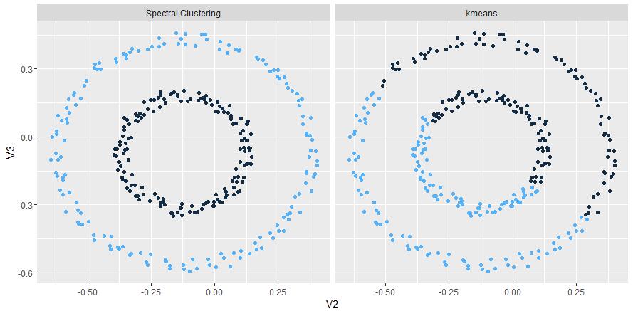

图12 spectral clustering和kmeans的对比

四、一些参考资料

Meila,shi: A Random Walks View of Spectral Segmentation
Harry Yserentant: A short theory of the Rayleigh-Ritz method
Ulrike von Luxburg: A Tutorial on Spectral Clustering
Andrew Y.Ng, Michael I.Jordan, Yair Weiss: On Spectral Clustering Analysis and an algorithm
L. LOVASZ: Random Walks on Graphs: A Survey
Fan R.K. Chung: Spectral Graph Theory
Xiao-Dong Zhang: The Laplacian eigenvalues of graphs: a survey
Bojan Mohar: THE LAPLACIAN SPECTRUM OF GRAPHS
pluskid: http://blog.pluskid.org/?p=287
Wiki: https://en.wikipedia.org/wiki/Jacobi_eigenvalue_algorithm
G. E. FORSYTHE AND P. HENRICI：THE CYCLIC JACOBI METHOD FOR COMPUTING THE PRINCIPAL VALUES OF A COMPLEX MATRIX
Jacobi Transformations of a Symmetric Matrix