TTSR(Learning Texture Transformer Network for Image Super-Resolution)论文及代码
文章目录前言一、Transformer二、Approach1.Texture Transformer( TT)2.Cross-Scale Feature Integration(CSFI)3.Loss Function总结前言主要记录个人对TTSR论文和代码的阅读,水平有限,欢迎指正论文——TTSRCVPR2020代码——CODE领域——超分辨率关键点——Reference-based Image
文章目录

前言
主要记录个人对TTSR论文和代码的阅读,水平有限,欢迎指正。
论文——TTSR(CVPR2020)
代码——CODE
领域——超分辨率
关键点——Reference-based Image Super-Resolution,Transfromer
相关解读——https://mp.weixin.qq.com/s/nPPbHHJmIc5amyKwJlCsUQ
https://blog.csdn.net/sinat_17456165/article/details/106678740
LR—低分辨率图片
HR—高分辨率图片
SR—超分辨率图片
REF—参考图片(高分辨率)
一、Transformer

Transfromer在NLP应用较多,最近在CV也进行了各种融合,详情查看
Transformer详解。
二、Approach
首先,提出了可学习的纹理提取器,其中的参数将在端到端训练过程中进行更新。这样的设计实现了低分辨率图像LR和参考Ref图像的联合特征嵌入,从而为在SR任务中应用注意机制奠定了坚实的基础。其次,提出一个相关嵌入模块来计算低分辨率图像LR和参考Ref图像之间的相关性。更具体地说,将从LR和Ref图像中提取的特征公式化为转换器中的查询和关键字,以获得硬注意力图和软注意力图。最后,提出了一个硬注意力模块和一个软注意力模块,以将高分辨率图HR特征从参考Ref图像转移并融合到通过注意力图从主干提取的LR特征中。因此,TTSR的设计了一种更精确的方法来搜索和从Ref图像转换为LR图像的相关纹理。此外,提出了一个跨尺度特征集成模块来堆叠纹理transformers,其中跨不同尺度(例如从1x到4x)学习特征以实现更强大的特征表示。
1.Texture Transformer( TT)

TT的结构如图2所示。 LR、LR↑和Ref分别表示输入图像、4×双三采样输入图像和参考图像。 依次在参考图像上应用具有相同因子的4×双三次下采样和上采样来获得Ref↓↑,使之与LR↑保持一致(domain-consistent是否还有其他含义?)。TT以Ref、Ref↓↑、LR↑和Backbone产生的LR特征作为输入,输出综合特征映射,用于进一步生成HR预测。
而代码和图并不是能很好地直接对应上,代码中model包含了TTSR.py,LTE.py,SearchTransfer.py,MainNet.py四个文件。
TT有四个部分:
可学习纹理提取器 learnable texture extractor (LTE)
相关性嵌入模块 relevance embedding module (RE)
特征转移硬注意模块 hard-attention module for feature transfer (HA)
特征合成软注意模块 soft-attention module for feature synthesis (SA)
TTSR code:
class TTSR(nn.Module):
    def __init__(self, args):
        super(TTSR, self).__init__()
        self.args = args
        self.num_res_blocks = list( map(int, args.num_res_blocks.split('+')) )
        self.MainNet = MainNet.MainNet(num_res_blocks=self.num_res_blocks, n_feats=args.n_feats,
            res_scale=args.res_scale)
        self.LTE      = LTE.LTE(requires_grad=True)
        self.LTE_copy = LTE.LTE(requires_grad=False) ### used in transferal perceptual loss
        self.SearchTransfer = SearchTransfer.SearchTransfer()

    def forward(self, lr=None, lrsr=None, ref=None, refsr=None, sr=None):
        if (type(sr) != type(None)):
            ### used in transferal perceptual loss
            self.LTE_copy.load_state_dict(self.LTE.state_dict())
            sr_lv1, sr_lv2, sr_lv3 = self.LTE_copy((sr + 1.) / 2.)
            return sr_lv1, sr_lv2, sr_lv3

        _, _, lrsr_lv3  = self.LTE((lrsr.detach() + 1.) / 2.)   #Q
        _, _, refsr_lv3 = self.LTE((refsr.detach() + 1.) / 2.)  #K
        ref_lv1, ref_lv2, ref_lv3 = self.LTE((ref.detach() + 1.) / 2.) #V

        S, T_lv3, T_lv2, T_lv1 = self.SearchTransfer(lrsr_lv3, refsr_lv3, ref_lv1, ref_lv2, ref_lv3)  #RE HA

        sr = self.MainNet(lr, S, T_lv3, T_lv2, T_lv1)  #Backbone  F S T SA

        return sr, S, T_lv3, T_lv2, T_lv1
其中残差块的数量,第一次转化的通道数等是作为超参传入的。
默认网络结构参数:
num_res_blocks = '16+16+8+4'
n_feats = 64
res_scale = 1
LTE(Learnable Texture Extractor)
使用LTE提取LR↑,Ref↓↑,Ref分别得到Q,K,V,其中Q和K只使用了第三级特征。
Q 为 Query,代表从低分辨率提取出的纹理特征信息,用来进行纹理搜索;K 为 Key,代表高分辨率参考图像经过先下采样再上采样得到的与低分辨率图像分布一致的图像的纹理信息,用来进行纹理搜索;V为 Value,代表原参考图像的纹理信息,用来进行纹理迁移。
LTE code:
#learnable textture extractor
class LTE(torch.nn.Module):
    def __init__(self, requires_grad=True, rgb_range=1):
        super(LTE, self).__init__()
        ### use vgg19 weights to initialize
        vgg_pretrained_features = models.vgg19(pretrained=True).features
        self.slice1 = torch.nn.Sequential()
        self.slice2 = torch.nn.Sequential()
        self.slice3 = torch.nn.Sequential()
        for x in range(2):
            self.slice1.add_module(str(x), vgg_pretrained_features[x])
        for x in range(2, 7):
            self.slice2.add_module(str(x), vgg_pretrained_features[x])
        for x in range(7, 12):
            self.slice3.add_module(str(x), vgg_pretrained_features[x])
        if not requires_grad:
            for param in self.slice1.parameters():
                param.requires_grad = requires_grad
            for param in self.slice2.parameters():
                param.requires_grad = requires_grad
            for param in self.slice3.parameters():
                param.requires_grad = requires_grad
        vgg_mean = (0.485, 0.456, 0.406)
        vgg_std = (0.229 * rgb_range, 0.224 * rgb_range, 0.225 * rgb_range)
        self.sub_mean = MeanShift(rgb_range, vgg_mean, vgg_std)
    def forward(self, x):
        x = self.sub_mean(x)
        x = self.slice1(x)
        x_lv1 = x
        x = self.slice2(x)
        x_lv2 = x
        x = self.slice3(x)
        x_lv3 = x
        return x_lv1, x_lv2, x_lv3
VGG每次池化步长为2,则x_lv1,x_lv2,x_lv3分别是输入图像/1,输入图像/2,输入图像/4。
对论文中的“Instead of using semantic features extracted by a pre-trained classification model like VGG , we design a learnable texture extractor whose parameters will be updated during end-to-end training.”存在疑惑,虽然说VGG会对特征进行降维得到高层级的语义信息,从而丢失了低层级的像素信息,但LTE在code中还是使用了VGG的前几层,可能意思是不加载预训练权重?
SearchTransfer
之后将LTE提取的纹理特征输入到SearchTransfer(ST),ST主要完成RE和HA运算。
SearchTransfer code:
class SearchTransfer(nn.Module):
    def __init__(self):
        super(SearchTransfer, self).__init__()

    def bis(self, input, dim, index):
        # batch index select
        # input: [N, ?, ?, ...]
        # dim: scalar > 0
        # index: [N, idx]
        views = [input.size(0)] + [1 if i!=dim else -1 for i in range(1, len(input.size()))]
        expanse = list(input.size())
        expanse[0] = -1
        expanse[dim] = -1
        index = index.view(views).expand(expanse)
        return torch.gather(input, dim, index)

    def forward(self, lrsr_lv3, refsr_lv3, ref_lv1, ref_lv2, ref_lv3):
        ### search
        lrsr_lv3_unfold  = F.unfold(lrsr_lv3, kernel_size=(3, 3), padding=1)    #Q
        refsr_lv3_unfold = F.unfold(refsr_lv3, kernel_size=(3, 3), padding=1)  #K
        refsr_lv3_unfold = refsr_lv3_unfold.permute(0, 2, 1)

        refsr_lv3_unfold = F.normalize(refsr_lv3_unfold, dim=2) # [N, Hr*Wr, C*k*k]
        lrsr_lv3_unfold  = F.normalize(lrsr_lv3_unfold, dim=1) # [N, C*k*k, H*W]

        # relevance embedding
        R_lv3 = torch.bmm(refsr_lv3_unfold, lrsr_lv3_unfold) #[N, Hr*Wr, H*W]
        R_lv3_star, R_lv3_star_arg = torch.max(R_lv3, dim=1) #[N, H*W]    #R_lv3_star S    R_lv3_star_arg H

        ### transfer
        ref_lv3_unfold = F.unfold(ref_lv3, kernel_size=(3, 3), padding=1)     #V
        ref_lv2_unfold = F.unfold(ref_lv2, kernel_size=(6, 6), padding=2, stride=2)
        ref_lv1_unfold = F.unfold(ref_lv1, kernel_size=(12, 12), padding=4, stride=4)


        # hard attention
        T_lv3_unfold = self.bis(ref_lv3_unfold, 2, R_lv3_star_arg)
        T_lv2_unfold = self.bis(ref_lv2_unfold, 2, R_lv3_star_arg)
        T_lv1_unfold = self.bis(ref_lv1_unfold, 2, R_lv3_star_arg)

        T_lv3 = F.fold(T_lv3_unfold, output_size=lrsr_lv3.size()[-2:], kernel_size=(3,3), padding=1) / (3.*3.)
        T_lv2 = F.fold(T_lv2_unfold, output_size=(lrsr_lv3.size(2)*2, lrsr_lv3.size(3)*2), kernel_size=(6,6), padding=2, stride=2) / (3.*3.)
        T_lv1 = F.fold(T_lv1_unfold, output_size=(lrsr_lv3.size(2)*4, lrsr_lv3.size(3)*4), kernel_size=(12,12), padding=4, stride=4) / (3.*3.)

        S = R_lv3_star.view(R_lv3_star.size(0), 1, lrsr_lv3.size(2), lrsr_lv3.size(3))

        return S, T_lv3, T_lv2, T_lv1
ST主要作用在于寻找可迁移纹理,RE将 Q 和 K 分别像卷积计算一样(unfold可以看做一种滑动窗口操作)提取出特征块,然后以内积(bmm)的方式计算 Q 和 K 中的特征块两两之间的相关性。内积越大的地方代表两个特征块之间的相关性越强,可迁移的高频纹理信息越多。反之,内积越小的地方代表两个特征块之间的相关性越弱,可迁移的高频纹理信息越少。相关性嵌入模块会输出一个硬注意力图和一个软注意力图。
其中,硬注意力图记录了对 Q 中的每一个特征块,K 中对应的最相关的特征块的位置;软注意力图记录了这个最相关的特征块的具体相关性,即内积大小。R_lv3_star_arg应用到硬注意力模块HA,而R_lv3_star应用到软注意力模块SA中。
HA中利用硬注意力图中所记录的位置,从 V 中迁移对应位置的特征块,进而组合成一个迁移纹理特征图 T。T 的每个位置包含了参考图像中最相似的位置的高频纹理特征。T 随后会与骨干网络中的特征进行通道级联和特征融合。图2中H的整数表示位置信息。
SA软注意力模块中,上述融合的特征会与软注意力图进行对应位置的点乘,相关性强的纹理信息能够赋予相对更大的权重;相关性弱的纹理信息,能够因小权重得到抑制。因此,软注意力模块能够使得迁移过来的高频纹理特征得到更准确的利用。图2中S的小数表示相关性权重大小。
另外,图2中左上角的运算符号由以下式子表示,运算符⊙表示特征映射之间的元素乘法,具体实现在MainNet中。
MainNet
代码中对SA的处理在MainNet中,MainNet 包括了图2中的LR,backbone,F和后续另说明的 Cross-Scale Feature Integration(CSFI),网络结构的可视化图参考下面CSFI中的图3。
MainNet code:
class MainNet(nn.Module):
    def __init__(self, num_res_blocks, n_feats, res_scale):
        super(MainNet, self).__init__()
        self.num_res_blocks = num_res_blocks ### a list containing number of resblocks of different stages
        self.n_feats = n_feats

        self.SFE = SFE(self.num_res_blocks[0], n_feats, res_scale)   # backbone

        ### stage11
        self.conv11_head = conv3x3(256+n_feats, n_feats)
        self.RB11 = nn.ModuleList()
        for i in range(self.num_res_blocks[1]):
            self.RB11.append(ResBlock(in_channels=n_feats, out_channels=n_feats,
                res_scale=res_scale))
        self.conv11_tail = conv3x3(n_feats, n_feats)

        ### subpixel 1 -> 2
        self.conv12 = conv3x3(n_feats, n_feats*4)
        self.ps12 = nn.PixelShuffle(2)

        ### stage21, 22
        #self.conv21_head = conv3x3(n_feats, n_feats)
        self.conv22_head = conv3x3(128+n_feats, n_feats)

        self.ex12 = CSFI2(n_feats)

        self.RB21 = nn.ModuleList()
        self.RB22 = nn.ModuleList()
        for i in range(self.num_res_blocks[2]):
            self.RB21.append(ResBlock(in_channels=n_feats, out_channels=n_feats,
                res_scale=res_scale))
            self.RB22.append(ResBlock(in_channels=n_feats, out_channels=n_feats,
                res_scale=res_scale))

        self.conv21_tail = conv3x3(n_feats, n_feats)
        self.conv22_tail = conv3x3(n_feats, n_feats)

        ### subpixel 2 -> 3
        self.conv23 = conv3x3(n_feats, n_feats*4)
        self.ps23 = nn.PixelShuffle(2)

        ### stage31, 32, 33
        #self.conv31_head = conv3x3(n_feats, n_feats)
        #self.conv32_head = conv3x3(n_feats, n_feats)
        self.conv33_head = conv3x3(64+n_feats, n_feats)

        self.ex123 = CSFI3(n_feats)

        self.RB31 = nn.ModuleList()
        self.RB32 = nn.ModuleList()
        self.RB33 = nn.ModuleList()
        for i in range(self.num_res_blocks[3]):
            self.RB31.append(ResBlock(in_channels=n_feats, out_channels=n_feats,
                res_scale=res_scale))
            self.RB32.append(ResBlock(in_channels=n_feats, out_channels=n_feats,
                res_scale=res_scale))
            self.RB33.append(ResBlock(in_channels=n_feats, out_channels=n_feats,
                res_scale=res_scale))

        self.conv31_tail = conv3x3(n_feats, n_feats)
        self.conv32_tail = conv3x3(n_feats, n_feats)
        self.conv33_tail = conv3x3(n_feats, n_feats)

        self.merge_tail = MergeTail(n_feats)

    def forward(self, x, S=None, T_lv3=None, T_lv2=None, T_lv1=None):
        ### shallow feature extraction
        x = self.SFE(x)

        ### stage11
        x11 = x

        ### soft-attention
        x11_res = x11
        x11_res = torch.cat((x11_res, T_lv3), dim=1)
        x11_res = self.conv11_head(x11_res) #F.relu(self.conv11_head(x11_res))
        x11_res = x11_res * S
        x11 = x11 + x11_res

        x11_res = x11

        for i in range(self.num_res_blocks[1]):
            x11_res = self.RB11[i](x11_res)
        x11_res = self.conv11_tail(x11_res)
        x11 = x11 + x11_res

        ### stage21, 22
        x21 = x11
        x21_res = x21
        x22 = self.conv12(x11)
        x22 = F.relu(self.ps12(x22))

        ### soft-attention
        x22_res = x22
        x22_res = torch.cat((x22_res, T_lv2), dim=1)
        x22_res = self.conv22_head(x22_res) #F.relu(self.conv22_head(x22_res))
        x22_res = x22_res * F.interpolate(S, scale_factor=2, mode='bicubic')
        x22 = x22 + x22_res

        x22_res = x22

        x21_res, x22_res = self.ex12(x21_res, x22_res)

        for i in range(self.num_res_blocks[2]):
            x21_res = self.RB21[i](x21_res)
            x22_res = self.RB22[i](x22_res)

        x21_res = self.conv21_tail(x21_res)
        x22_res = self.conv22_tail(x22_res)
        x21 = x21 + x21_res
        x22 = x22 + x22_res

        ### stage31, 32, 33
        x31 = x21
        x31_res = x31
        x32 = x22
        x32_res = x32
        x33 = self.conv23(x22)
        x33 = F.relu(self.ps23(x33))

        ### soft-attention
        x33_res = x33
        x33_res = torch.cat((x33_res, T_lv1), dim=1)
        x33_res = self.conv33_head(x33_res) #F.relu(self.conv33_head(x33_res))
        x33_res = x33_res * F.interpolate(S, scale_factor=4, mode='bicubic')
        x33 = x33 + x33_res

        x33_res = x33

        x31_res, x32_res, x33_res = self.ex123(x31_res, x32_res, x33_res)

        for i in range(self.num_res_blocks[3]):
            x31_res = self.RB31[i](x31_res)
            x32_res = self.RB32[i](x32_res)
            x33_res = self.RB33[i](x33_res)

        x31_res = self.conv31_tail(x31_res)
        x32_res = self.conv32_tail(x32_res)
        x33_res = self.conv33_tail(x33_res)
        x31 = x31 + x31_res
        x32 = x32 + x32_res
        x33 = x33 + x33_res

        x = self.merge_tail(x31, x32, x33)

        return x
以下为Backbone实现
Backbone code:
class SFE(nn.Module):
    def __init__(self, num_res_blocks, n_feats, res_scale):
        super(SFE, self).__init__()
        self.num_res_blocks = num_res_blocks
        self.conv_head = conv3x3(3, n_feats)

        self.RBs = nn.ModuleList()
        for i in range(self.num_res_blocks):
            self.RBs.append(ResBlock(in_channels=n_feats, out_channels=n_feats,
                res_scale=res_scale))

        self.conv_tail = conv3x3(n_feats, n_feats)

    def forward(self, x):
        x = F.relu(self.conv_head(x))
        x1 = x
        for i in range(self.num_res_blocks):
            x = self.RBs[i](x)
        x = self.conv_tail(x)
        x = x + x1
        return x
以下为残差模块的实现,通过res_scale控制残差传递的权重。
ResBlock code:
class ResBlock(nn.Module):
    def __init__(self, in_channels, out_channels, stride=1, downsample=None, res_scale=1):
        super(ResBlock, self).__init__()
        self.res_scale = res_scale
        self.conv1 = conv3x3(in_channels, out_channels, stride)
        self.relu = nn.ReLU(inplace=True)
        self.conv2 = conv3x3(out_channels, out_channels)

    def forward(self, x):
        x1 = x
        out = self.conv1(x)
        out = self.relu(out)
        out = self.conv2(out)
        out = out * self.res_scale + x1
        return out
2.Cross-Scale Feature Integration(CSFI)
MainNet中很大一部分即是图三所表示的网络结构,存在大量残差块和线路交错,三个输入分别是之前寻找到的纹理T_lv3,T_lv2,T_lv1。将所提出的纹理Transformer 应用于 x1、x2、x4 三个不同的层级,并将不同层级间的特征通过上采样或带步长的卷积进行交叉融合。通过上述方式,不同粒度的参考图像信息会渗透到不同的层级,从而使得网络的特征表达能力增强,提高生成图像的质量。

第一个CSFI模块,融合x1和x2两级的特征。
CSFI2 code:
class CSFI2(nn.Module):
    def __init__(self, n_feats):
        super(CSFI2, self).__init__()
        self.conv12 = conv1x1(n_feats, n_feats)
        self.conv21 = conv3x3(n_feats, n_feats, 2)

        self.conv_merge1 = conv3x3(n_feats*2, n_feats)
        self.conv_merge2 = conv3x3(n_feats*2, n_feats)

    def forward(self, x1, x2):
        x12 = F.interpolate(x1, scale_factor=2, mode='bicubic')
        x12 = F.relu(self.conv12(x12))
        x21 = F.relu(self.conv21(x2))

        x1 = F.relu(self.conv_merge1( torch.cat((x1, x21), dim=1) ))
        x2 = F.relu(self.conv_merge2( torch.cat((x2, x12), dim=1) ))

        return x1, x2
第二个CSFI模块,融合x1,x2,x3三级特征。
CSFI3 code:
class CSFI3(nn.Module):
    def __init__(self, n_feats):
        super(CSFI3, self).__init__()
        self.conv12 = conv1x1(n_feats, n_feats)
        self.conv13 = conv1x1(n_feats, n_feats)

        self.conv21 = conv3x3(n_feats, n_feats, 2)
        self.conv23 = conv1x1(n_feats, n_feats)

        self.conv31_1 = conv3x3(n_feats, n_feats, 2)
        self.conv31_2 = conv3x3(n_feats, n_feats, 2)
        self.conv32 = conv3x3(n_feats, n_feats, 2)

        self.conv_merge1 = conv3x3(n_feats*3, n_feats)
        self.conv_merge2 = conv3x3(n_feats*3, n_feats)
        self.conv_merge3 = conv3x3(n_feats*3, n_feats)

    def forward(self, x1, x2, x3):
        x12 = F.interpolate(x1, scale_factor=2, mode='bicubic')
        x12 = F.relu(self.conv12(x12))
        x13 = F.interpolate(x1, scale_factor=4, mode='bicubic')
        x13 = F.relu(self.conv13(x13))

        x21 = F.relu(self.conv21(x2))
        x23 = F.interpolate(x2, scale_factor=2, mode='bicubic')
        x23 = F.relu(self.conv23(x23))

        x31 = F.relu(self.conv31_1(x3))
        x31 = F.relu(self.conv31_2(x31))
        x32 = F.relu(self.conv32(x3))

        x1 = F.relu(self.conv_merge1( torch.cat((x1, x21, x31), dim=1) ))
        x2 = F.relu(self.conv_merge2( torch.cat((x2, x12, x32), dim=1) ))
        x3 = F.relu(self.conv_merge3( torch.cat((x3, x13, x23), dim=1) ))

        return x1, x2, x3
最后的特征融合并输出SR图像。
MergeTail code:
class MergeTail(nn.Module):
    def __init__(self, n_feats):
        super(MergeTail, self).__init__()
        self.conv13 = conv1x1(n_feats, n_feats)
        self.conv23 = conv1x1(n_feats, n_feats)
        self.conv_merge = conv3x3(n_feats*3, n_feats)
        self.conv_tail1 = conv3x3(n_feats, n_feats//2)
        self.conv_tail2 = conv1x1(n_feats//2, 3)

    def forward(self, x1, x2, x3):
        x13 = F.interpolate(x1, scale_factor=4, mode='bicubic')
        x13 = F.relu(self.conv13(x13))
        x23 = F.interpolate(x2, scale_factor=2, mode='bicubic')
        x23 = F.relu(self.conv23(x23))

        x = F.relu(self.conv_merge( torch.cat((x3, x13, x23), dim=1) ))
        x = self.conv_tail1(x)
        x = self.conv_tail2(x)
        x = torch.clamp(x, -1, 1)

        return x
3.Loss Function
损失函数包括三部分——重建损失,对抗损失,感知损失,权重分别为λrec = 1,λadv = 1e-3,λper = 1e-2。
3.1 重建损失
直接对比SR与HR的像素差值,论文证明L1比L2表现的更清晰和收敛更快。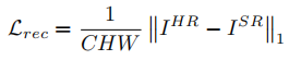
class ReconstructionLoss(nn.Module):
    def __init__(self, type='l1'):
        super(ReconstructionLoss, self).__init__()
        if (type == 'l1'):
            self.loss = nn.L1Loss()
        elif (type == 'l2'):
            self.loss = nn.MSELoss()
        else:
            raise SystemExit('Error: no such type of ReconstructionLoss!')

    def forward(self, sr, hr):
        return self.loss(sr, hr)
3.2 对抗损失
论文采用WGAN-GP,以梯度范数的惩罚来取代权重裁剪来获得更稳定的训练和更好的表现。
D(x)为图像真假二分类判别网络,十层卷积层加两层全连接层,不包含BN层,共进行了五次下采样。
λ在文中取10。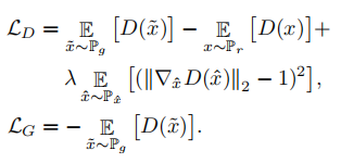
class AdversarialLoss(nn.Module):
    def __init__(self, logger, use_cpu=False, num_gpu=1, gan_type='WGAN_GP', gan_k=1,
        lr_dis=1e-4, train_crop_size=40):
        super(AdversarialLoss, self).__init__()
        self.logger = logger
        self.gan_type = gan_type
        self.gan_k = gan_k
        self.device = torch.device('cpu' if use_cpu else 'cuda')
        self.discriminator = discriminator.Discriminator(train_crop_size*4).to(self.device)
        self.optimizer = optim.Adam(self.discriminator.parameters(),betas=(0, 0.9), eps=1e-8, lr=lr_dis

        self.bce_loss = torch.nn.BCELoss().to(self.device)
        self.bcewithlogits_loss = torch.nn.BCEWithLogitsLoss().to(self.device)

    def forward(self, fake, real):
        fake_detach = fake.detach()

        for _ in range(self.gan_k):
            self.optimizer.zero_grad()
            d_fake = self.discriminator(fake_detach)
            d_real = self.discriminator(real)
            if (self.gan_type.find('WGAN') >= 0):
                loss_d = (d_fake - d_real).mean()
                if self.gan_type.find('GP') >= 0:
                    epsilon = torch.rand(real.size(0), 1, 1, 1).to(self.device)
                    epsilon = epsilon.expand(real.size())
                    hat = fake_detach.mul(1 - epsilon) + real.mul(epsilon)
                    hat.requires_grad = True
                    d_hat = self.discriminator(hat)
                    gradients = torch.autograd.grad(
                        outputs=d_hat.sum(), inputs=hat,
                        retain_graph=True, create_graph=True, only_inputs=True
                    )[0]
                    gradients = gradients.view(gradients.size(0), -1)
                    gradient_norm = gradients.norm(2, dim=1)
                    gradient_penalty = 10 * gradient_norm.sub(1).pow(2).mean()
                    loss_d += gradient_penalty


            # Discriminator update
            loss_d.backward()
            self.optimizer.step()

        d_fake_for_g = self.discriminator(fake)
        if (self.gan_type.find('WGAN') >= 0):
            loss_g = -d_fake_for_g.mean()

        # Generator loss
        return loss_g
3.3感知损失
感知损失用于增强预测图像与目标图像在特征空间上的相似性,文中包括了两部分,第一部分是SR和HR在VGG19上的特征图L2差异,第二部分计算SR和T特征图的L2差异。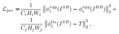
可见第一部分是从VGG19的第五块计算的MSE。
class PerceptualLoss(nn.Module):
    def __init__(self):
        super(PerceptualLoss, self).__init__()

    def forward(self, sr_relu5_1, hr_relu5_1):
        loss = F.mse_loss(sr_relu5_1, hr_relu5_1)
        return loss
第二部分称为转移感知损失,计算SR在LTE上的特征图和T(T是Figure 2上HR的转移纹理特征)的差异,由于之前的LTE产生了三级特征,文中使用求平均来处理。
class TPerceptualLoss(nn.Module):
    def __init__(self, use_S=True, type='l2'):
        super(TPerceptualLoss, self).__init__()
        self.use_S = use_S
        self.type = type

    def gram_matrix(self, x):
        b, ch, h, w = x.size()
        f = x.view(b, ch, h*w)
        f_T = f.transpose(1, 2)
        G = f.bmm(f_T) / (h * w * ch)
        return G

    def forward(self, map_lv3, map_lv2, map_lv1, S, T_lv3, T_lv2, T_lv1):
        ### S.size(): [N, 1, h, w]
        if (self.use_S):
            S_lv3 = torch.sigmoid(S)
            S_lv2 = torch.sigmoid(F.interpolate(S, size=(S.size(-2)*2, S.size(-1)*2), mode='bicubic'))
            S_lv1 = torch.sigmoid(F.interpolate(S, size=(S.size(-2)*4, S.size(-1)*4), mode='bicubic'))
        else:
            S_lv3, S_lv2, S_lv1 = 1., 1., 1.

        if (self.type == 'l1'):
            loss_texture  = F.l1_loss(map_lv3 * S_lv3, T_lv3 * S_lv3)
            loss_texture += F.l1_loss(map_lv2 * S_lv2, T_lv2 * S_lv2)
            loss_texture += F.l1_loss(map_lv1 * S_lv1, T_lv1 * S_lv1)
            loss_texture /= 3.
        elif (self.type == 'l2'):
            loss_texture  = F.mse_loss(map_lv3 * S_lv3, T_lv3 * S_lv3)
            loss_texture += F.mse_loss(map_lv2 * S_lv2, T_lv2 * S_lv2)
            loss_texture += F.mse_loss(map_lv1 * S_lv1, T_lv1 * S_lv1)
            loss_texture /= 3.

        return loss_texture
三、Experiments
数据集使用CUFED,实验放大倍数为x4,通过随机水平和垂直翻转来增强训练图像,然后随机旋转90°、180°和270◦。 每个batch包含9个LR补丁(大小为40×40),以及9个HR和Ref补丁(大小为160×160)。前两个epoch只使用Lrec重建损失,之后加上另外两个训练到50 epoch。
论文分别对HA,SA,LTE,CFFI等进行了消融实验。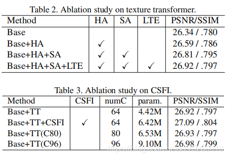

有“AI”的1024 = 2048,欢迎大家加入2048 AI社区
更多推荐
 14
14 0
0- 0


 已为社区贡献2条内容

所有评论(0)