此示例提供了使用k-Wave模拟和检测二维均匀传播介质中初始压力分布产生的压力场的简单演示。

本文是作者对程序的一些粗俗理解，如有错误欢迎更正~

有兴趣的同好可以加企鹅群交流：937503951，任何科研相关问题都可以在群内交流，平常一起聊聊天、分享日常也是没问题的，欢迎~

目录

一、打开官方示例程序

二、均匀传播介质程序的逐步理解

2.1 创建网格

2.2 定义介质

2.3 定义初始压力分布/定义声源

2.4 定义传感器

2.5 模拟仿真

三、绘图/数据可视化

3.1 绘制初始压力和传感器分布图

3.2 绘制传感器数据图/数据可视化

---

 

一、打开官方示例程序

注：官方文档中建议k-Wave新手优先完成初始值问题实例【Initial Value Problems】，再去学习特定领域的示例

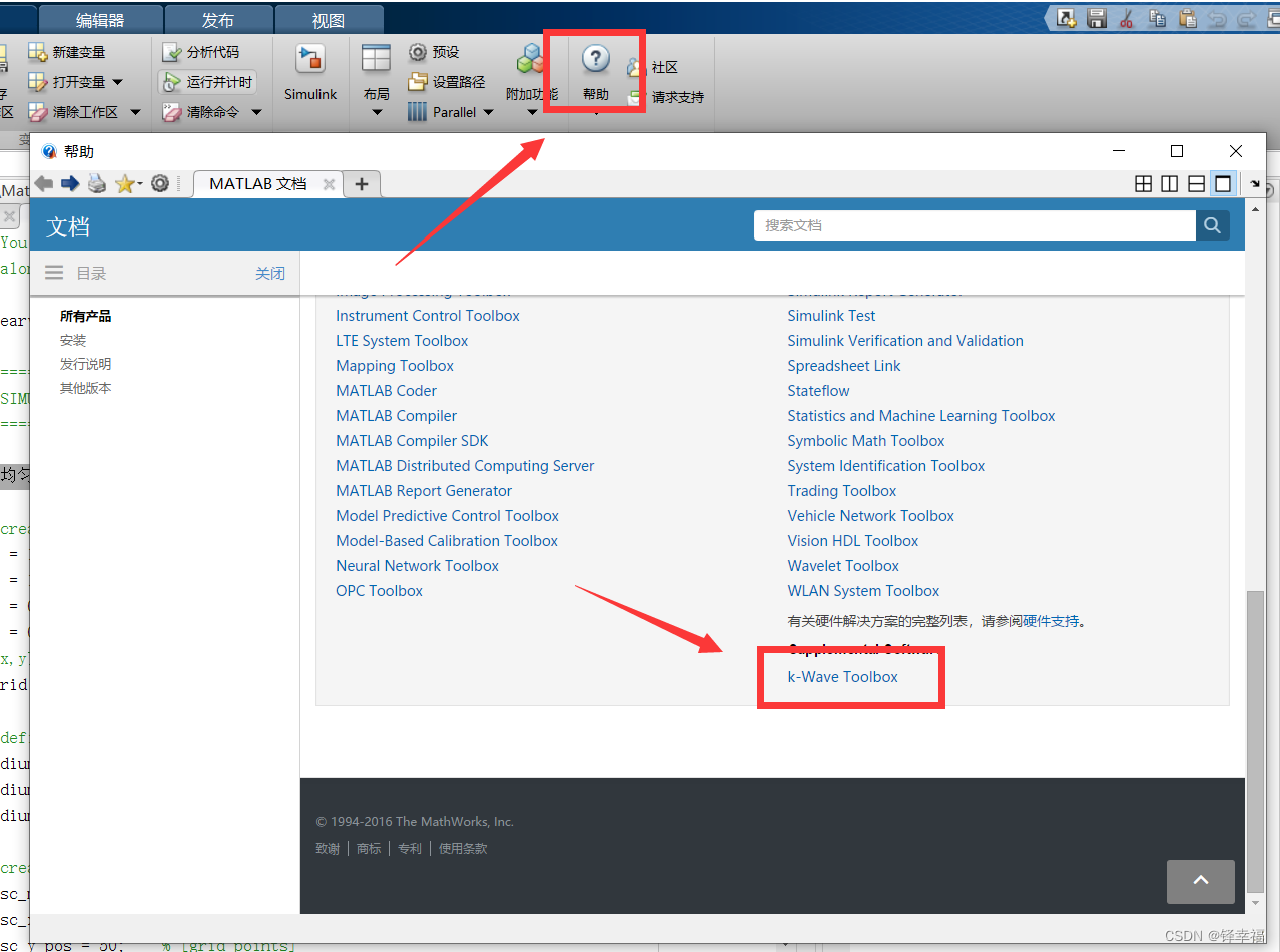
1.打开MATLAB【主页】-【帮助】，滑到下方点击【k-Wave Toolbox】

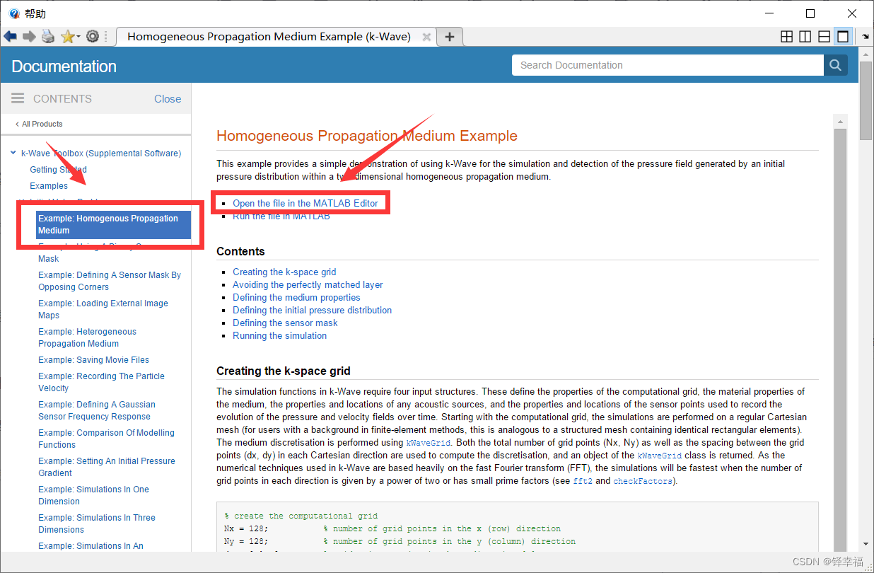
2.找到官方的第一个示例，选择在MATLAB中打开【Open the file in the MATLAB Editor】

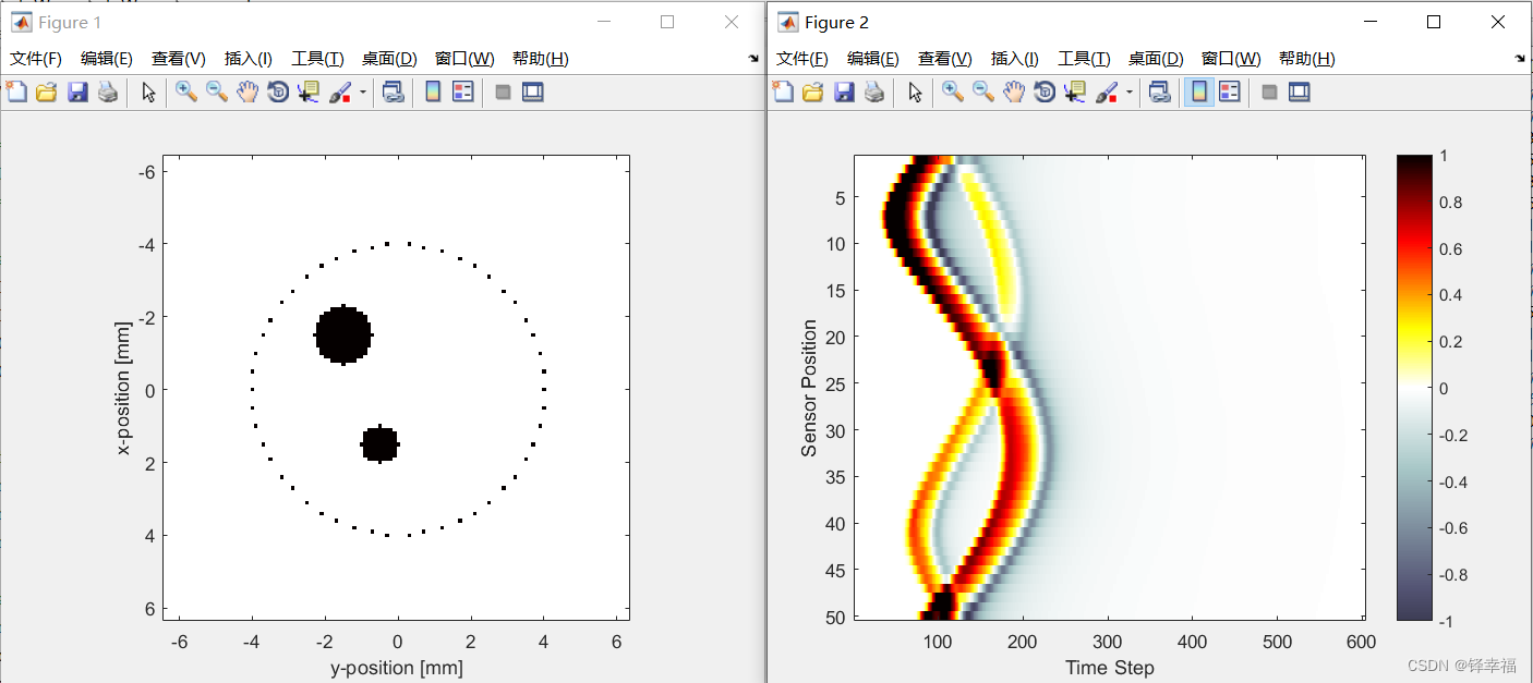
3.直接【运行】一下，查看结果：一幅动图过后，绘制出两幅图（数据可视化）

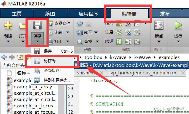
4.可以选择将文件在【编辑器】-【保存】-【另存为】中将示例文件另存为新文件，在不影响官方示例原程序的基础上，方便根据自己需求更改与注释程序

 

二、均匀传播介质程序的逐步理解

2.1 创建网格

% create the computational grid
Nx = 128;           % number of grid points in the x (row) direction
Ny = 128;           % number of grid points in the y (column) direction
dx = 0.1e-3;        % grid point spacing in the x direction [m]
dy = 0.1e-3;        % grid point spacing in the y direction [m]
kgrid = kWaveGrid(Nx, dx, Ny, dy);

Nx与Ny为x和y方向网格的数量，这里均为128；

dx与dy为x和y方向网格的大小，为0.1*10^(-3) [m]，也就是0.1[mm]；

所以，所建网格的横纵坐标轴长度=128*0.1(数量*大小)=12.8[mm]，所以在【Figure 1】中可以看到横纵坐标轴都为(-6.4 , 6.4)。

kgrid = kWaveGrid(Nx, dx, Ny, dy); %绘制网格函数

ps.官方提示：Avoiding the perfectly matched layer(避免使用完美匹配的图层) —— 这里不太懂，以后再说0.q

waves as they get close to the edge of the computational domain. By default, this layer occupies a strip of 20 grid points (10 grid points in 3D) around the edge of the domain inside the computational domain specified using kWaveGrid. To avoid strange effects, care must be taken not to place the source or sensor points inside this layer. Alternatively, the perfectly matched layer can be set to be outside the computational domain set by the user. See Controlling The Absorbing Boundary Layer Example for more detailed instructions on how to modify the properties and position of the perfectly matched layer.

当声波到达计算域的边缘时，它们被一种特殊类型的各向异性吸收边界层吸收，称为完美匹配层 （PML）。通过观察传播波在接近计算域边缘时会发生什么，可以看出该层的影响。默认情况下，此图层在使用指定的计算域内围绕域边缘的20个网格点（3D中为10个网格点）占据一条带状。为避免奇怪的效果，必须注意不要将源或传感器点放置在该层内。或者，可以将完美匹配的层设置为用户设置的计算域之外。有关如何修改完美匹配层的属性和位置的更详细说明，请参阅控制吸收边界层示例。

 

2.2 定义介质

% define the properties of the propagation medium
medium.sound_speed = 1500;  % [m/s]
medium.alpha_coeff = 0.75;  % [dB/(MHz^y cm)]
medium.alpha_power = 1.5;

定义声速等一些参数。

Power law acoustic absorption(幂律吸声)可以通过给medium.alpha_coeff和medium.alpha_power幅值来设置 —— 这里不太明白，只知道是参数设置。

 

2.3 定义初始压力分布/定义声源

% create initial pressure distribution using makeDisc
disc_magnitude = 5; % [Pa]
disc_x_pos = 50;    % [grid points]
disc_y_pos = 50;    % [grid points]
disc_radius = 8;    % [grid points]
disc_1 = disc_magnitude * makeDisc(Nx, Ny, disc_x_pos, disc_y_pos, disc_radius);

disc_magnitude = 3; % [Pa]
disc_x_pos = 80;    % [grid points]
disc_y_pos = 60;    % [grid points]
disc_radius = 5;    % [grid points]
disc_2 = disc_magnitude * makeDisc(Nx, Ny, disc_x_pos, disc_y_pos, disc_radius);

source.p0 = disc_1 + disc_2;

这里创建了两个不同半径的圆形初始压力分布，所以在【Figure 1】中可以看到两个黑色圆形。

初始压力分布设置为一个矩阵，其中包含每个网格点的初始压力值，此矩阵的大小必须与第一步定义网格的大小相同。

disc_magnitude = 5; % 压力大小，单位[Pa]
disc_x_pos = 50;      % x坐标为50*0.1[mm]=5[mm]，因为是从-6.4开始，所以x坐标大概为-1.4[mm]
disc_y_pos = 50;      % 同y坐标
disc_radius = 8;        % 半径为8*0.1[mm]=0.8[mm]；另一个初始压力分布(声源)计算方法一致
disc_1 = disc_magnitude * makeDisc(Nx, Ny, disc_x_pos, disc_y_pos, disc_radius);
%makeDisc为在2D网格中创建二进制映射，可以简单理解为在网格中画出压力分布图(声源图)；用压力*makeDisc得到第一个压力分布(声源)

source.p0 = disc_1 + disc_2; %将两个压力分布(声源)相加，完成定义

ps.也可通过加载外部图像映射来定义初始压力分布(声源)，详见：k-Wave丨光声成像仿真丨其他方式定义传感器、声源+定义异构介质并可视化（三）-CSDN博客

 

2.4 定义传感器

% define a centered circular sensor
sensor_radius = 4e-3;   % [m]
num_sensor_points = 50;
sensor.mask = makeCartCircle(sensor_radius, num_sensor_points);

sensor_radius = 4e-3;       %传感器半径：4*10^(-3)[m] = 4mm
num_sensor_points = 50; %传感器数量：50
sensor.mask = makeCartCircle(sensor_radius, num_sensor_points); %可以理解为在网格图中画出这50个传感器，默认圆心在网格图正中央，【Figure 1】中那一圈小黑点就是传感器

ps.也可以通过其他两个方法定义传感器：使用二进制定义传感器和通过对角定义传感器，详见：k-Wave丨光声成像仿真丨其他方式定义传感器、声源+定义异构介质并可视化（三）-CSDN博客

 

2.5 模拟仿真

% run the simulation
sensor_data = kspaceFirstOrder2D(kgrid, medium, source, sensor);

kspaceFirstOrder2D函数中参数的顺序就是书写程序的顺序：定义网格、介质、声源、传感器

 

三、绘图/数据可视化

3.1 绘制初始压力和传感器分布图

figure;
imagesc(kgrid.y_vec * 1e3, kgrid.x_vec * 1e3, source.p0 + cart2grid(kgrid, sensor.mask), [-1, 1]);
colormap(getColorMap);
ylabel('x-position [mm]');
xlabel('y-position [mm]');
axis image;

把【Figure 1】放在这里，方便对照程序——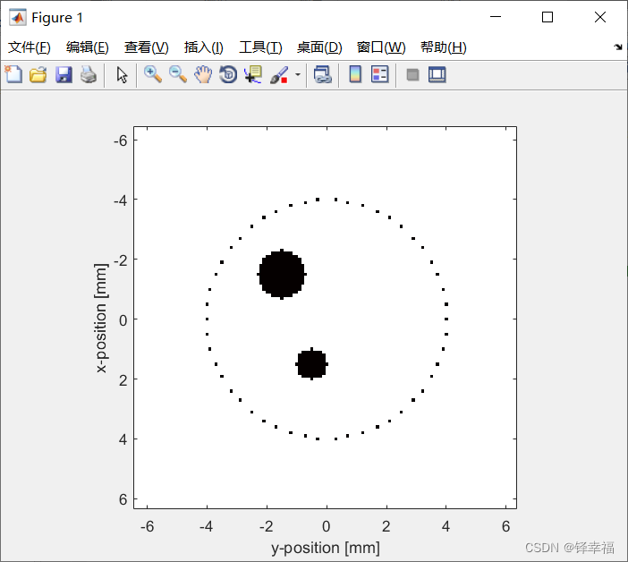

figure; %创建绘图板
imagesc(kgrid.y_vec * 1e3, kgrid.x_vec * 1e3, source.p0 + cart2grid(kgrid, sensor.mask), [-1, 1]);
% 以下是个人理解，存在偏差，不过在初期可以便于理解——
% imagesc为绘制颜色图函数
% kgrid.y_vec * 1e3和kgrid.x_vec * 1e3分别为绘出纵横坐标，*1e3的目的是将单位m变为mm
% vec：将向量转换为标量，即将绘制网格时的矩阵量变为绘图需要的标量
% source.p0 + cart2grid(kgrid, sensor.mask)为绘出声源(两个黑色圆形)和传感器(一圈黑色小点)
% cart2grid：将一组笛卡尔点插值到二进制网格上，也就是把传感器的坐标点都绘制出来
% 数据线性映射到[-1,1]之间，然后使用当前设置的颜色表进行显示，此时的[-1,1]充满了整个颜色表。
% 如果不写上[-1, 1]会使图片变成带颜色的，不是常规的k-Wave颜色(这里是黑白色)
colormap(getColorMap);
% getColorMap：返回默认的k-Wave颜色映射，没有这一步也是会使图片变成带颜色的，应该是和上面的[-1, 1]搭配使用的
ylabel('x-position [mm]'); %y坐标轴标题
xlabel('y-position [mm]'); %x坐标轴标题
axis image;                     %使xy坐标轴比例大小一致，不然绘制出的图是扁的，适用于图像显示

3.2 绘制传感器数据图/数据可视化

% plot the simulated sensor data
figure;
imagesc(sensor_data, [-1, 1]);
colormap(getColorMap);
ylabel('Sensor Position');
xlabel('Time Step');
colorbar;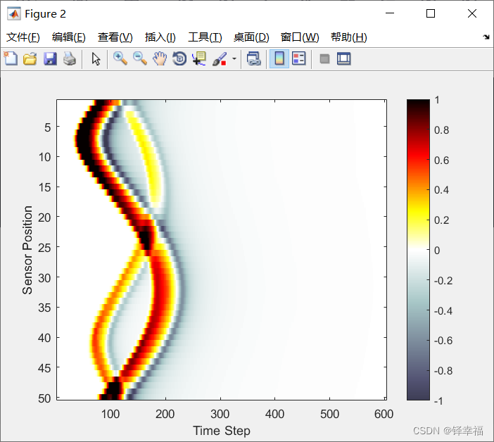

figure;
imagesc(sensor_data, [-1, 1]); %绘制传感器数据，只有sensor_data这一组数据，也是需要加上[-1, 1]
colormap(getColorMap);          %同上
ylabel('Sensor Position');         %同上
xlabel('Time Step');                  %同上
colorbar;                                  %显示图像的颜色条，最右边的长条