深度学习(斋藤)学习笔记(一)
深度学习入门-基于python的理论与实现,学习笔记系列,包括:学习心得与代码实践
·
激活函数
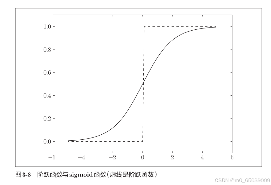
sigmoid函数
# coding: utf-8
import numpy as np
import matplotlib.pylab as plt
def sigmoid(x):
return 1 / (1 + np.exp(-x))
X = np.arange(-5.0, 5.0, 0.1)
Y = sigmoid(X)
plt.plot(X, Y)
plt.ylim(-0.1, 1.1)
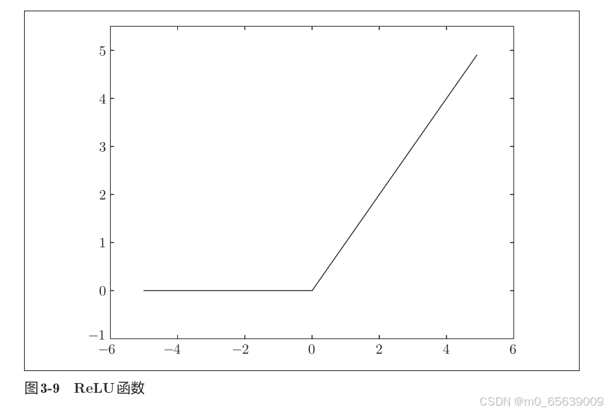
plt.show()relu函数
# coding: utf-8
import numpy as np
import matplotlib.pylab as plt
def relu(x):
return np.maximum(0, x)
x = np.arange(-5.0, 5.0, 0.1)
y = relu(x)
plt.plot(x, y)
plt.ylim(-1.0, 5.5)
plt.show()神经网络
import numpy as np
def sigmoid(x):
return 1 / (1 + np.exp(-x))
def identity_function(x):
return x
def init_network():
network = {}
network['W1'] = np.array([[0.1, 0.3, 0.5],
[0.2, 0.4, 0.6]])
network['b1'] = np.array([0.1, 0.2, 0.3])
network['W2'] = np.array([[0.1, 0.4],
[0.2, 0.5],
[0.3, 0.6]])
network['b2'] = np.array([0.1, 0.2])
network['W3'] = np.array([[0.1, 0.3],
[0.2, 0.4]])
network['b3'] = np.array([0.1, 0.2])
return network
def forward(network, x):
W1, W2, W3 = network['W1'], network['W2'], network['W3']
b1, b2, b3 = network['b1'], network['b2'], network['b3']
a1 = np.dot(x, W1) + b1
z1 = sigmoid(a1)
a2 = np.dot(z1, W2) + b2
z2 = sigmoid(a2)
a3 = np.dot(z2, W3) + b3
y = identity_function(a3)
return y
# 初始化网络并测试
network = init_network()
x = np.array([1.0, 0.5])
y = forward(network, x)
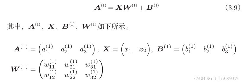
print(y) # 输出: [0.31682708 0.69627909]输出层
输出最后结果y的identity_function:恒等函数和 softmax 函数(解决分类问题)

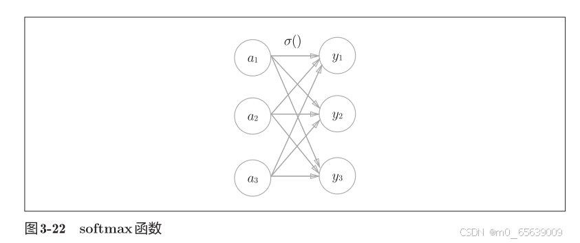
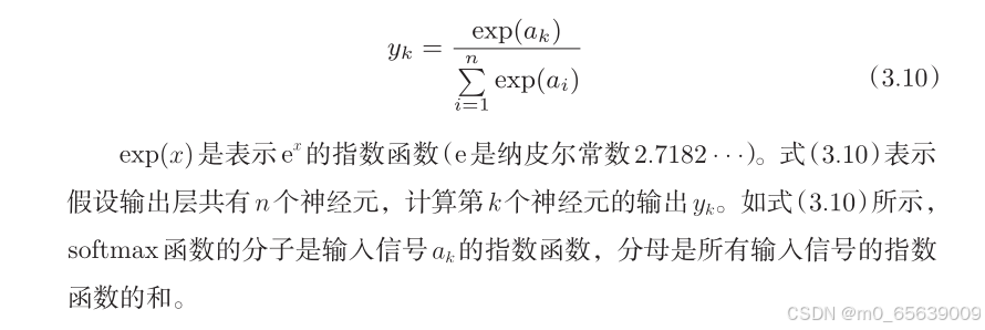
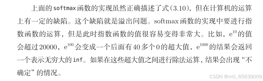
解决方法
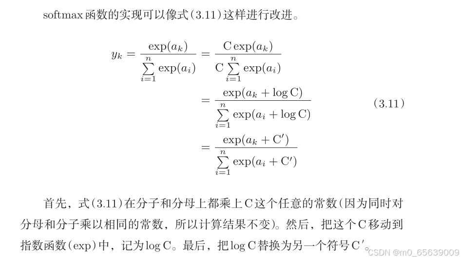
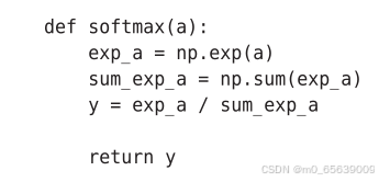
def softmax(a):
    c = np.max(a)
    exp_a = np.exp(a - c) # 溢出对策
    sum_exp_a = np.sum(exp_a)
    y = exp_a / sum_exp_a
    return y
实战
数据预处理
import torch
from torchvision import datasets, transforms
from torch.utils.data import DataLoader
import numpy as np
def load_mnist(normalize=True, flatten=True, one_hot_label=False, batch_size=64):
"""
加载 MNIST 数据集,并根据传入的参数进行处理。
参数:
- normalize: 是否将图像的像素值归一化到 [0, 1] 区间,默认是 True。
- flatten: 是否将图像展平为一维数组,默认是 True(784个元素的向量)。
- one_hot_label: 是否将标签转为 one-hot 表示,默认是 False。
- batch_size: 数据加载的批次大小,默认为 64。
返回:
- (训练集图像, 训练集标签),(测试集图像, 测试集标签)
"""
# 定义数据预处理(转换)
transform_list = []
if normalize:
transform_list.append(transforms.ToTensor()) # 转换为 Tensor
transform_list.append(transforms.Normalize((0.5,), (0.5,))) # 标准化
else:
transform_list.append(transforms.ToTensor()) # 只做转换为 Tensor,不进行归一化
transform = transforms.Compose(transform_list)
# 下载训练数据集
train_dataset = datasets.MNIST(root='./data', train=True, download=True, transform=transform)
# 下载测试数据集
test_dataset = datasets.MNIST(root='./data', train=False, download=True, transform=transform)
# 使用 DataLoader 加载数据集(分批次加载)
train_loader = DataLoader(train_dataset, batch_size=batch_size, shuffle=True)
test_loader = DataLoader(test_dataset, batch_size=batch_size, shuffle=False)
# 获取一个批次的数据
def get_data(loader):
images, labels = next(iter(loader))
if flatten:
images = images.view(-1, 28 * 28) # 展平图像
if one_hot_label:
labels = torch.eye(10)[labels] # 将标签转换为 one-hot 表示
return images, labels
train_images, train_labels = get_data(train_loader)
test_images, test_labels = get_data(test_loader)
return (train_images, train_labels), (test_images, test_labels)
# 测试代码
if __name__ == '__main__':
(train_images, train_labels), (test_images, test_labels) = load_mnist(normalize=True, flatten=True,
one_hot_label=True)
print(f"训练集图像形状: {train_images.shape}")
print(f"训练集标签形状: {train_labels.shape}")
print(f"测试集图像形状: {test_images.shape}")
print(f"测试集标签形状: {test_labels.shape}")
img=train_images[0]
tool=transforms.ToPILImage()
img=tool(img.squeeze(0).reshape(28,28))
img.show()在代码中,作为一种预处理,我们将各个像素值除以 255,进行了简单的正规化。实际上,很多预处理都会考虑到数据的整体分布。比如,利用数据整体的均值或标准差,移动数据,使数据整体以 0 为中心分布,或者进行正规化,把数据的延展控制在一定范围内。除此之外,还有将数据整体的分布形状均匀化的方法,即数据白化(whitening)等。
神经网络的推理处理
输入层有 784 个神经元,输出层有 10 个神经元。输入层的 784 这个数字来源于图像大小的 28 × 28 = 784,输出层的 10 这个数字来源于 10 类别分类(数字 0 到 9,共 10 类别)。此外,这个神经网络有 2 个隐藏层,第 1 个隐藏层有50 个神经元,第 2 个隐藏层有 100 个神经元。这个 50 和 100 可以设置为任何值。
import numpy as np
import pickle
import os
from scipy.special import softmax
# 在另一个脚本中导入
from dataprocess import load_mnist
def init_network():
# 检查是否存在已保存的权重文件
if os.path.exists("sample_weight.pkl"):
# 如果文件存在,加载权重文件
with open("sample_weight.pkl", 'rb') as f:
network = pickle.load(f)
print("加载了预训练的权重。")
else:
# 如果文件不存在,随机初始化网络权重
network = {}
network['W1'] = np.random.randn(784, 50) # 输入到隐藏层的权重
network['b1'] = np.zeros(50) # 隐藏层的偏置
network['W2'] = np.random.randn(50, 100) # 隐藏层到输出层的权重
network['b2'] = np.zeros(100) # 输出层的偏置
network['W3'] = np.random.randn(100, 10) # 隐藏层到输出层的权重
network['b3'] = np.zeros(10) # 输出层的偏置
# 将网络结构保存到.pkl文件
with open("sample_weight.pkl", 'wb') as f:
pickle.dump(network, f)
print("初始化了网络并保存权重。")
return network
# Sigmoid 激活函数
def sigmoid(x):
return 1 / (1 + np.exp(-x))
# 获取测试数据
def get_data():
(x_train, t_train), (x_test, t_test) = load_mnist(normalize=True, flatten=True, one_hot_label=False)
return x_test, t_test
# 预测函数
def predict(network, x):
W1, W2, W3 = network['W1'], network['W2'], network['W3']
b1, b2, b3 = network['b1'], network['b2'], network['b3']
# 第一层计算
a1 = np.dot(x, W1) + b1
z1 = sigmoid(a1)
# 第二层计算
a2 = np.dot(z1, W2) + b2
z2 = sigmoid(a2)
# 第三层计算
a3 = np.dot(z2, W3) + b3
y = softmax(a3) # 使用 softmax 激活函数得到输出的概率分布
return y # 返回预测的概率分布
# 进行预测并输出结果
def main():
# 获取数据
x_test, t_test = get_data()
# 初始化网络
network = init_network()
# 对测试集中的每一张图片进行预测
correct_count = 0
for i in range(len(x_test)):
# 对每个测试样本进行预测
y = predict(network, x_test[i])
# 获取预测的类别(概率最大的那个)
predicted_label = np.argmax(y)
# 获取实际标签
true_label = t_test[i]
# 比较预测的标签和真实标签,统计正确的预测次数
if predicted_label == true_label:
correct_count += 1
# 输出准确率
accuracy = correct_count / len(x_test) * 100
print(f"Test accuracy: {accuracy:.2f}%")
# 运行主程序
if __name__ == "__main__":
main()运行结果:
![]()
可以看到准确率很低,这是由于没有损失函数与方向传播,下一篇我们将学习损失函数,计算图,梯度与反向传播。

有“AI”的1024 = 2048,欢迎大家加入2048 AI社区
更多推荐


 40
40 0
0- 0


 已为社区贡献11条内容

所有评论(0)